15. Exploring Optimization and Scaling of Large Language Models

15. Exploring Optimization and Scaling of Large Language Models

In this chapter, we move from optimizing individual training runs to making cost–performance decisions for large-scale models.

Large Language Models represent one of the most demanding workloads ever deployed on modern computing systems. Their training pushes hardware, software stacks, and system architectures to their limits—not only in terms of raw computational throughput, but also in memory capacity, communication efficiency, energy consumption, and economic cost.

In the previous chapters, we established the foundations required to understand how large-scale training is executed on supercomputing platforms: GPU architectures, parallel execution models, deep learning frameworks, and distributed runtimes. In this chapter, we bring all those elements together and focus on a central question:

How should an HPC practitioner reason about the optimization and scaling of LLM training workloads?

Rather than presenting optimization as a checklist of techniques, this chapter adopts a system-centric perspective. Each experiment is designed to reveal why a given optimization helps, when its benefits diminish, and what trade-offs it introduces.

Although the chapter follows a practical and experimental approach, the optimizations explored are not arbitrary. They are implicitly guided by a small set of recurring ideas about how performance behaves in large-scale training systems. In this chapter, these ideas are made explicit in the form of a set of Foundational Performance Principles, which will be used as informal conceptual references throughout the experimental analysis.

Importantly, the goal of this chapter is not to maximize absolute performance at all costs. In real production and research environments, optimization decisions are constrained by hardware availability, budget, development effort, and operational complexity. Consequently, this chapter emphasizes decision-making over raw benchmarking, encouraging the reader to interpret results critically rather than mechanically applying every possible optimization.

To keep the focus on systems behavior rather than model accuracy, all experiments are conducted using a fixed model configuration and synthetic data. This controlled setup allows us to isolate the impact of architectural choices, numerical precision, kernel implementations, and parallel execution strategies—making the observed performance trends easier to interpret and generalize.

By the end of this chapter, the reader should not only be familiar with a set of concrete optimization techniques, but also be able to reason about which optimizations make sense for a given context, when scaling is justified, and how performance, efficiency, and cost interact in large-scale LLM training.

How to Read This Chapter

This chapter is structured as a progressive exploration of optimization and scaling decisions, rather than as a linear recipe to be followed blindly. Each section builds upon the previous one, revealing how performance bottlenecks shift as the system configuration evolves.

Readers are encouraged to focus not only on the numerical results, but on the trends and breakpoints observed in each experiment. In several cases, an optimization that delivers clear benefits in one configuration provides diminishing or negligible returns in another. These transitions are intentional and reflect real-world system behavior.

While the experiments are executed on a specific supercomputing platform, the underlying principles are broadly applicable. The objective is not to replicate identical performance numbers on other systems, but to acquire a transferable mental model for optimizing and scaling LLM workloads in diverse HPC environments.

Foundational Performance Principles

Throughout this book, a set of recurring ideas has been progressively introduced to explain how performance emerges in high performance computing systems and, more recently, in large-scale deep learning workloads. In earlier chapters, these ideas appeared in different contexts—GPU execution, distributed training, memory behavior, and pipeline analysis—each time addressing a specific aspect of system behavior. In this chapter, they are brought together explicitly as a unified conceptual framework.

These ideas are referred to as Foundational Performance Principles. They describe structural regularities that consistently appear when training deep learning models at scale and provide a common language for reasoning about performance phenomena that are often treated in an ad hoc or fragmented manner in practice.

Importantly, these principles are not intended to form a hierarchy, nor to be applied in a fixed or sequential order. None of them supersedes or invalidates the others. Instead, they capture different but complementary constraints that shape performance in large-scale training systems. Depending on the workload, hardware, and execution context, different principles may become more visible or more limiting, but all remain simultaneously active.

These principles should also not be interpreted as optimization recipes or as a prescriptive methodology. Their purpose is different. They aim to capture fundamental constraints that govern the behavior of large-scale training systems, independently of the specific frameworks, libraries, or hardware generations used at any given time.

A key characteristic of these principles is that they do not depend on a particular GPU architecture or deep learning framework. Instead, they arise from fundamental limitations related to data movement, communication, memory usage, and computational cost. As a result, while optimization techniques evolve rapidly—new kernels, new parallelization strategies, or new runtimes—the principles that justify them remain largely stable.

In this book, the Foundational Performance Principles are organized into four complementary categories, each reflecting a different level of reasoning about system behavior.

#1: Amortization of Overheads (Operational)

Any training system incurs fixed and recurring costs, such as initialization, synchronization, kernel launches, or control overheads. Performance depends on how effectively these costs are amortized relative to useful computation. Increasing batch size, increasing work per iteration, or running for sufficient duration are common mechanisms through which overheads become negligible in steady-state execution.

#2: Hardware–Software Co-Design Matters (Architectural)

Training performance is strongly influenced by the alignment between software behavior and hardware characteristics, including compute units, memory hierarchies, interconnects, and specialized execution units. While overhead amortization, pipeline balance, and scaling efficiency are often evaluated through metrics such as throughput and utilization, hardware–software co-design explains why those metrics can approach—or remain far from—their theoretical limits. In this sense, co-design acts as an enabling principle: it defines the performance envelope within which the other principles operate.

#3: Balanced Pipelines (Systemic)

End-to-end training performance emerges from the interaction of multiple pipeline stages, spanning data access, preprocessing, memory movement, computation, and coordination. A single dominant bottleneck is sufficient to limit overall system throughput, regardless of optimizations applied elsewhere. While both overhead amortization and pipeline balance address underutilization, they operate at different conceptual levels: the former focuses on reducing the relative cost of fixed expenses, whereas the latter ensures that no continuously active stage throttles sustained throughput.

#4: Scale Must Serve Purpose (Decisional)

Scaling is not an objective in itself. Increasing the number of resources only makes sense in relation to an explicit goal, such as reducing time-to-solution, meeting a deadline, maximizing throughput, or optimizing cost or energy efficiency. This principle should be understood as decisional rather than technical. It does not replace the other principles, nor does it resolve performance limitations by itself. Instead, it provides the context in which the outcomes revealed by overhead amortization, pipeline balance, and hardware–software co-design are interpreted and acted upon.

Taken together, these four principles form a coherent mental framework. Operational principles explain how performance is achieved, architectural principles explain its limits, systemic principles explain its stability under load, and decisional principles explain how performance should be evaluated and used in practice.

In the remainder of this chapter, these principles are used informally as guiding ideas while exploring a sequence of optimization and scaling steps for training a large language model. The focus remains on observing system behavior, interpreting measurements, and understanding trade-offs, rather than on applying a formal or prescriptive optimization procedure.

Case Study and Code

This chapter is built around a single, controlled case study designed to expose the dominant performance behaviors encountered when training Large Language Models on modern supercomputing platforms. Rather than continuously changing models, datasets, or training objectives, we deliberately fix these elements to isolate the impact of system-level optimization decisions.

The selected models—LLaMA 3.2 and OPT—are representative of contemporary transformer-based architectures, while remaining tractable for systematic experimentation. To further simplify analysis, all experiments rely on synthetic data. This choice removes variability introduced by data loading, preprocessing, or I/O bottlenecks, allowing us to focus exclusively on computation, memory usage, and communication behavior.

It is important to emphasize that the purpose of this baseline configuration is not to achieve state-of-the-art accuracy or training efficiency. Instead, it serves as a diagnostic reference point. By starting from a simple, unoptimized setup, we can clearly observe how each subsequent optimization affects system behavior—and when its benefits begin to saturate.

From a performance perspective, this baseline configuration should be understood as an intentionally low-inertia operating point. Fixed overheads, memory pressure, and synchronization costs are not yet amortized, making their impact on training throughput clearly observable. This deliberate choice allows the optimization steps explored in the following sections to expose how different system-level decisions progressively shift the dominant performance constraints.

The baseline training script introduced in this section will be reused throughout the chapter with minimal modifications. This continuity is intentional: performance differences observed in later sections can be attributed directly to specific optimization choices, rather than to changes in model structure or training logic.

LLaMA 3.2 1B and OPT 1.3B Models

This section introduces the practical foundation for the optimization and scaling experiments discussed throughout the chapter. We will work with two real-world large language models: the open-source LLaMA 3.2 1B-parameter model (Llama-3.2-1B) with 1 billion parameters, and OPT 1.3B model (facebook/opt-1.3b), a 1.3B-parameter model from the OPT family.

While both models are considered small by today’s LLM standards, they preserve the core architectural and computational characteristics of much larger transformers, making them especially well suited for controlled benchmarking, optimization studies, and scaling experiments on modern GPU-based HPC systems (including MareNostrum 5). Throughout this chapter, we will present and analyze the experimental results obtained with LLaMA 3.2 1B, while students will be asked to reproduce the same experiments using OPT 1.3B and compare both behaviors.

Both models were obtained from the Hugging Face Model Hub. For the teaching laboratories associated with this book, the models are pre-downloaded and transferred to the shared filesystem of the supercomputing platform to facilitate classroom execution. Readers working in other environments can instead download the models directly from Hugging Face, following the same procedure introduced in the previous chapter.

Synthetic Data

To emphasize computational performance rather than model accuracy, we use a synthetic dataset of 10,000 samples generated dynamically. This approach removes variability introduced by I/O operations or preprocessing, ensuring that performance metrics reflect the computational efficiency of the training process. This method is common in benchmarking studies, allowing us to focus on GPU utilization, training throughput, and memory usage without interference from data loading bottlenecks.

Baseline Training Script

We establish a baseline using the Python script benchmark.py, which trains the LLaMA 3.2 model on a single GPU using Hugging Face’s Trainer API, putting into practice the layered architecture and execution flow illustrated in Figure 13.5.

This script collects essential performance metrics, serving as a reference point for evaluating the impact of optimizations explored in later sections.

In summary, the benchmark.py script:

Defines model precision (either bf16 or fp32) to evaluate memory efficiency and numerical stability.
Loads a pretrained model (AutoModelForCausalLM) from HF.
Generates a synthetic dataset (DummyDataset).
Initializes the Trainer API with appropriate training arguments.
Logs key performance metrics, including Training Throughput and Max Reserved GPU Memory.

The code listing is as follows:

import os
import torch

from transformers import AutoModelForCausalLM, Trainer
from utils import DummyDataset, get_args, log_rank, report_memory

def main(training_arguments, benchmark_arguments):
    # Set the data type for model parameters (bf16 or fp32)
    TORCH_DTYPE = torch.bfloat16 if benchmark_arguments.model_precision == "bf16" 
                                 else torch.float
    world_size = int(os.environ["WORLD_SIZE"])

    model = AutoModelForCausalLM.from_pretrained(
        benchmark_arguments.path_to_model,
        attn_implementation=benchmark_arguments.attn,
        torch_dtype=TORCH_DTYPE
    )

    train_dataset = DummyDataset(
        benchmark_arguments.sequence_length,
        benchmark_arguments.num_samples
    )

    trainer = Trainer(
        model=model,
        args=training_arguments,
        train_dataset=train_dataset
    )

    metrics = trainer.train().metrics
            log_rank(f"Training throughput:    {training_arguments.max_steps *    
            training_arguments.per_device_train_batch_size * 
            benchmark_arguments.sequence_length/metrics['train_runtime']:.2f} 
            Tokens/s/GPU")
    
    report_memory()

if __name__ == "__main__":
    _training_arguments, _benchmark_arguments = get_args()
    main(_training_arguments, _benchmark_arguments)

The utils.py module, used in conjunction with this script, provides utility functions and classes and should reside in the same directory. No modifications are required.

The baseline configuration presented here should be interpreted as a starting point for reasoning, not as a recommended production setup. In high performance environments, meaningful optimization requires first understanding where time, memory, and resources are being spent. A transparent baseline provides that reference, making subsequent performance gains—and their limitations—both measurable and interpretable.

Performance Metrics: Measuring Training Efficiency

This script collects two key metrics:

Training Throughput (Tokens/s/GPU): Quantifies the speed at which tokens are processed. It is calculated as:
Max Reserved GPU Memory (GB): Obtained using torch.cuda.max_memory_reserved(), this value indicates peak memory usage during training.

These metrics allow us to evaluate how different configurations affect efficiency and scalability.

Example output from a baseline run:

INFO -> Training throughput:     27542.25 Tokens/s/GPU
INFO -> Max reserved GPU Memory: 61.59

SLURM Job Submission Script

As in Chapters 11 and 12, we use torchrun in a SLURM environment. The Python code now relies on the Hugging Face Trainer API, but the job launcher strategy remains familiar. The SLURM script is available in the GitHub repository accompanying this book.

To explore performance systematically, only a few variables need to be modified in the SLURM submission script. The following variables are fixed to ensure consistency across experiments:

MAX_STEPS: Maximum number of training steps.
SEQUENCE_LEN: Input sequence length in tokens. (Kept short to accommodate course resource limitations.)
OPTIMIZER: Optimizer used; fixed to AdamW.
TORCH_COMPILE: Whether to use torch.compile. When using LIGER_KERNEL=true, TORCH_COMPILE must remain disabled.

The variables to be changed across experiments include:

MICRO_BATCH_SIZE: Number of samples per device in each forward/backward pass.
MODEL_PRECISION: Precision format (fp32, bf16).
MIXED_PRECISION: Enables AMP (Automatic Mixed Precision).
ATTN: Attention implementation: eager, sdpa, flash_attention_2.
LIGER_KERNEL: Whether optimized kernels are used.

These will be introduced in detail in each subsequent experiment.

Running the Baseline Experiment

We begin by running the experiment with the default SLURM script:

#!/bin/bash
#SBATCH --job-name <your_job_name>
#SBATCH --chdir . # local directory
#SBATCH --output ./results/R-%x.%j.out  
#SBATCH --error ./results/R-%x.%j.err  

#SBATCH --nodes <nodes>                    
#SBATCH --ntasks-per-node 1         
#SBATCH --gres gpu: <num_gpus>                
#SBATCH --cpus-per-task 20          
#SBATCH --time 00:29:59  

           
#SBATCH --account <account>
#SBATCH --qos acc_debug
#SBATCH --exclusive

GPUS_PER_NODE=1  # between 1 and 4 GPUs to inform torchrun
MICRO_BATCH_SIZE= <batch_size>
MODEL_PRECISION="fp32" # bf16 - fp32
MIXED_PRECISION="no" # bf16 - fp8 - no
ATTN=eager # eager - flash_attention_2 - sdpa
LIGER_KERNEL=false # false - true 

module load singularity

MASTER_ADDR=$(scontrol show hostnames $SLURM_JOB_NODELIST | head -n 1)
MASTER_PORT=6000

LAUNCHER="torchrun \
    --nproc_per_node $GPUS_PER_NODE \
    --nnodes $SLURM_NNODES \
    --node_rank \$SLURM_PROCID \
    --rdzv_endpoint $MASTER_ADDR:$MASTER_PORT \
    --rdzv_backend c10d \
    --max_restarts 0 \
    --tee 3 \
    "

PATH_TO_MODEL= <path_to_model>
MODEL= <name>  # LLAMA3.2-1B or facebook/opt-1.3b 

MAX_STEPS=450
SEQUENCE_LEN=1024
OPTIMIZER=adamw_torch 
TORCH_COMPILE=false 

RUN_NAME="NODES-$SLURM_NNODES-GPUs-$GPUS_PER_NODE-$MODEL-MODEL-PRECISION-$MODEL_PRECISION-MIXED-PRECISION-$MIXED_PRECISION-ATTN-$ATTN-$OPTIMIZER-TC-$TORCH_COMPILE-LIGER-$LIGER_KERNEL-SEQLEN-$SEQUENCE_LEN-MBS-mak$MICRO_BATCH_SIZE-$(cat /proc/sys/kernel/random/uuid)"

PYTHON_FILE=<path>/benchmark.py
PYTHON_ARGS="--path_to_model $PATH_TO_MODEL \
    --run_name $RUN_NAME \
    --max_steps $MAX_STEPS \
    --sequence_length $SEQUENCE_LEN \
    --per_device_train_batch_size $MICRO_BATCH_SIZE \
    --model_precision $MODEL_PRECISION \
    --attn $ATTN \
    --torch_compile $TORCH_COMPILE \
    --use_liger_kernel $LIGER_KERNEL \
    --optim $OPTIMIZER \
    --output_dir ./results/output \
    --save_strategy no \
    --report_to none \
     "

export CMD="ACCELERATE_MIXED_PRECISION=$MIXED_PRECISION $LAUNCHER $PYTHON_FILE $PYTHON_ARGS"

SINGULARITY_CONTAINER=/gpfs/apps/MN5/ACC/SINGULARITY/SRC/images/nvidiaPytorch24.07_bis.sif

SINGULARITY_ARGS=" \
    --nv \
    $SINGULARITY_CONTAINER \
    "

SRUN_ARGS=" \
    --cpus-per-task $SLURM_CPUS_PER_TASK \
    --jobid $SLURM_JOB_ID \
    "

echo "$CMD"
srun $SRUN_ARGS bsc_singularity exec  $SINGULARITY_ARGS bash -c "$CMD"

Results are recorded in a Table 15.1 that tracks the value of each variable per run.

Task	Num GPUs	Batch Size	Model Precision	Mixed Precision	Attention Type	Liger	Training Throughput	Memory (GB)
15.1	1	6	fp32	No	eager	false	10,485	61.89

Table 15.1 – Baseline training results using LLaMA 3.2 1B model.

Task 15.1 – Baseline Experiments

Replicate the baseline training experiment for the LLaMA 3.2 1B (Llama-3.2-1B) and OPT 1.3B (facebook/opt-1.3b), which were downloaded in the previous chapter, using the default hyperparameters defined in the SLURM file according to Table 15.1, without applying any memory-saving techniques, kernel optimizations, or distributed execution.

For this baseline run, record:

training throughput,

GPU memory usage,

time per training step or iteration.

Do not attempt to optimize performance at this stage. The goal of this task is not to obtain good performance, but to establish a reference point against which all subsequent optimizations will be evaluated.

For this initial baseline, it is recommended to start with a batch size of 6 for LLaMA 3.2 1B and a batch size of 4 for OPT 1.3B, as a safe initial configuration to ensure stable execution.

All the exercises in this chapter are designed to be carried out exclusively by modifying the SLURM job scripts. The SLURM template can be obtained from GitHub, and no Python files need to be modified.

Proceed as follows:

First, run the experiment with the LLaMA-based configuration to verify that you obtain results consistent with those reported in this chapter.

Then, repeat exactly the same procedure using the OPT-based configuration.

Then, answer explicitly:

What limits performance in this baseline configuration?

Which resources appear to be under pressure (compute, memory capacity, memory bandwidth)?

Summarize your observations clearly stating what this baseline reveals about the initial constraints of the system.

With this baseline established, the following sections will progressively explore optimization strategies applied to the same training workflow. As we will see, not all optimizations deliver uniform benefits, and some introduce new constraints or trade-offs. Understanding why these effects occur is central to developing sound intuition for large-scale LLM training on supercomputing systems.

Efficient Training on a Single GPU

Before scaling training across multiple GPUs or nodes, it is essential to fully understand the performance envelope of a single accelerator. A modern GPU such as the NVIDIA H100 already embodies massive parallelism, deep memory hierarchies, and highly specialized execution units. As a result, many of the performance phenomena observed at scale are already present—and often easier to interpret—at the single-GPU level.

As discussed in Chapter 11, training throughput is strongly influenced by factors such as batch size, numerical precision, and the efficiency of critical kernel implementations. In this section, we conduct a sequence of controlled experiments aimed at progressively exposing the limits of single-GPU training performance. Rather than treating optimization as a checklist, each experiment is designed to reveal which resource becomes the bottleneck as configuration parameters change.

All experiments are executed on a single NVIDIA H100 GPU using the same baseline model and training script introduced in Section 15.2. This controlled setup allows us to reason clearly about memory pressure, computational efficiency, and hardware utilization—laying a solid foundation for the multi-GPU scaling analysis that follows later.

We begin by exploring batch size scaling under full precision, and then progressively introduce mixed precision, full model precision, optimized attention kernels, and Triton-based Liger kernels. Each step illustrates how different layers of the hardware–software stack interact to shape the achievable performance envelope.

Batch Size Scaling

Batch size scaling is often presented as a straightforward way to improve GPU utilization. In performance terms, its role is more fundamental: it is the simplest controlled intervention that reveals whether the training workflow is operating in an overhead-dominated regime. By increasing the amount of useful work performed per step, we can observe how fixed and recurring costs—such as framework overhead, kernel launch overheads, and per-step control logic—are amortized, and identify the point at which memory capacity or sustained compute becomes the dominant constraint.

In our SLURM scripts, the batch size is controlled using the MICRO_BATCH_SIZE variable, which determines the number of samples processed per GPU in each forward and backward pass. By progressively increasing this value, we can observe how fixed per-step costs are amortized and identify the point at which memory constraints dominate execution.

This first sequence of experiments is a direct reappearance of Foundational Performance Principle #1 (Amortization of Overheads). As micro-batch size grows, fixed and recurring costs—kernel launches, framework bookkeeping, and per-step runtime overheads—are amortized over more useful work. The result is not only higher throughput, but also a clearer separation between regimes where performance is dominated by “setup and overhead” versus regimes where it is dominated by sustained computation.

As batch size increases, the training workload transitions from an overhead-dominated regime to a computation-dominated regime—a shift that is fundamental to understanding why scaling can be effective, but also why it eventually saturates.

We begin with a conservative batch size and incrementally increase it until the GPU runs out of memory (OOM). This trial-and-error process reveals the memory limit and serves as a baseline for further optimizations.

Task	Num GPUs	Batch Size	Model Precision	Mixed Precision	Attention Type	Liger	Training Throughput	Memory (GB)
15.1	1	6	fp32	No	eager	false	10,485	61.89
15.2	1	7	fp32	No	eager	false	-	OOM

Table 15.2 – Training throughput and memory usage for the baseline training configuration on a single GPU, serving as the reference point for subsequent optimizations.

Task 15.2 – Finding the Out-of-Memory (OOM) Limit

Starting from the baseline configuration in Task 15.1, progressively increase the batch size until the training run fails due to an out-of-memory (OOM) error.

Proceed in two stages:

First, perform this experiment with LLaMA 3.2 1B to verify that you correctly understand the methodology and can reliably identify the OOM point.

Then, repeat exactly the same procedure with OPT 1.3B.

For each attempted configuration, record:

batch size,

GPU memory usage,

whether execution succeeds or fails.

Identify the maximum viable batch size, defined as the largest batch size that can be executed without exceeding GPU memory capacity.

Finally, compare and discuss both results. What differences do you observe between LLaMA 3.2 1B and OPT 1.3B? How does the increase from 1B to 1.3B parameters reflect on the attainable batch size and memory pressure?

The batch size experiments presented above establish a first, crucial boundary: the memory ceiling imposed by full-precision training on a single GPU. While increasing batch size improves throughput up to a point, it also reveals how quickly modern LLM workloads exhaust available memory resources. This observation motivates the next set of experiments, where numerical precision becomes the primary lever for unlocking additional performance headroom.

Enhancing Training Efficiency with Mixed Precision

Mixed precision is often introduced as a way to reduce memory usage and enable larger batch sizes. While this is sometimes true, it is not the main reason why mixed precision is so effective on modern GPUs. In many large language model workloads—especially those operating close to the device memory limit—mixed precision should be understood primarily as a hardware alignment strategy: it changes how the same training computation maps onto the GPU’s specialized execution units and memory hierarchy.

This set of experiments is a direct illustration of Foundational Performance Principle #2 (Hardware–Software Co-Design). Numerical precision is not merely a numerical choice; it selects different kernel implementations, activates matrix engines such as Tensor Cores, and reshapes the balance between compute throughput and memory traffic. As a result, the same high-level training algorithm can exhibit substantially different performance characteristics depending on how precision is configured.

Mixed precision training (introduced in Chapter 11) combines lower-precision computation with selective higher-precision storage to accelerate training while preserving numerical stability. In this chapter, we use bfloat16 (bf16), which provides a wider dynamic range than fp16 and typically avoids the need for loss scaling. On NVIDIA H100 GPUs, bf16 enables efficient Tensor Core execution and can increase throughput with minimal changes to the training workflow.

To activate mixed precision, we set the MIXED_PRECISION variable in the SLURM script. In this configuration, model computation is performed in bf16, while selected components—most notably optimizer states—remain in fp32 to preserve numerical robustness.

Although mixed precision is often associated with reduced memory usage and increased batch size, this expectation does not always hold in practice—particularly for large language models trained close to the Out-of-Memory boundary. While activations and gradients do benefit directly from reduced precision, they represent only a fraction of the total memory footprint during training.

A dominant share of GPU memory is consumed by optimizer states, especially when using adaptive optimizers such as AdamW. For each model parameter, AdamW maintains additional tensors to store first and second moments, which are typically kept in fp32 for numerical stability, regardless of the precision used for model weights and activations. As a result, a substantial portion of memory usage remains unaffected by mixed precision.

Beyond optimizer states, GPU memory is also consumed by temporary CUDA buffers, framework runtime allocations, communication workspaces, and internal tensor conversions. On H100-class GPUs, enabling bf16 activates different kernel implementations and execution paths, which may introduce additional transient buffers. When training operates close to the physical memory limit of the device, these secondary effects—although individually small—can become decisive and trigger an Out-of-Memory condition earlier than anticipated.

In our experiments, switching from fp32 to bf16 mixed precision allows training with a batch size of five—just below the OOM threshold—while delivering modest memory savings and a measurable increase in throughput. This outcome illustrates a key point: mixed precision improves performance primarily by increasing computational efficiency, not by uniformly reducing memory consumption.

For this reason, mixed precision should be understood first and foremost as a compute-side optimization. Its benefits arise from faster matrix operations, improved utilization of specialized execution units, and better amortization of compute-bound kernels, rather than from a guaranteed expansion of the memory ceiling.

Task	Num GPUs	Batch Size	Model Precision	Mixed Precision	Attention Type	Liger	Training Throughput	Memory (GB)
15.3	1	5	fp32	bf16	eager	false	11,489	58.27

Table 15.3 – Training with mixed precision (bf16) reduces memory consumption and increases throughput.

Memory fragmentation further complicates this picture. The dynamic allocation and deallocation of tensors during forward and backward passes can lead to non-contiguous free memory regions. Even when the total amount of free memory appears sufficient, fragmentation may prevent the allocation of a large contiguous block required for a new batch, again resulting in an OOM error. This effect becomes increasingly pronounced as training approaches the physical memory limits of the GPU.

For these reasons, it is entirely possible—and common in practice—that activating bf16 mixed precision improves throughput while leaving the maximum achievable batch size unchanged, or even slightly reduced, compared to fp32. Mixed precision should therefore be understood primarily as a performance optimization technique, not as a guaranteed mechanism for increasing batch size.

Its real benefits emerge from faster computation, improved hardware utilization, and better amortization of compute-bound kernels, rather than from a uniform reduction of the overall memory footprint. Recognizing this distinction is essential when reasoning about optimization strategies for large-scale LLM training. In other words, once overheads have been partially amortized through batch size scaling, precision becomes one of the most effective levers to raise the compute intensity of each step.

Task 15.3 – Mixed Precision Training

Starting from the configuration used in Task 15.2, modify the SLURM script to enable bf16 mixed precision by activating the MIXED_PRECISION variable. Use this configuration to evaluate the impact of mixed precision on training throughput and GPU memory consumption.

Proceed again in two stages:

First, run the experiment with LLaMA 3.2 1B using the same hyperparameters reported in this chapter, and verify that your results are consistent with the reference measurements in terms of throughput, memory usage, and stability.

Then, repeat exactly the same experiment with OPT 1.3B.

As part of this experiment, progressively increase the batch size again under bf16 precision until you reach the new OOM limit. Note that, despite using mixed precision, it may still be necessary to reduce the batch size with respect to fp32 for stability reasons, depending on the memory pressure introduced by the optimizer and activation checkpoints.

For both models, record data obtained.

Finally, compare and discuss the results obtained with LLaMA 3.2 1B and OPT 1.3B. In particular¹:

How does mixed precision change the memory footprint of the training process?

Does mixed precision lead to similar throughput improvements for both models?

Does the maximum batch size under bf16 decrease in both cases?

How does the difference in parameter count (1B vs. 1.3B) reflect on memory usage and attainable batch size under mixed precision?

Fine-Tuning Model Precision

Beyond mixed precision, memory pressure can be reduced further by lowering the numerical precision of the entire model. Unlike mixed precision training—which preserves fp32 master weights—this approach stores model parameters, activations, and gradients directly in bfloat16 format. By eliminating high-precision replicas, the training workflow undergoes a structural reduction in its memory footprint.

This distinction is critical. While mixed precision primarily changes how computation is executed, full bf16 model precision changes how the model itself is represented in memory. As a result, the memory savings achieved at this stage are qualitatively different from those obtained through mixed precision and translate more directly into additional headroom for batch size scaling or runtime buffers.

From a systems perspective, this optimization again reflects Foundational Performance Principle #2 (Hardware–Software Co-Design Matters). By aligning the numerical representation of the model with the native execution format of modern GPUs, both memory traffic and storage requirements are reduced. In our experiments on the NVIDIA H100, enabling full bf16 model precision produces a substantial reduction in memory usage—close to 10 GB—together with a noticeable increase in training throughput. This shift alleviates pressure on the memory subsystem and moves execution further toward a compute-efficient regime.

Despite this additional headroom, the achievable batch size remains constrained by other components of the training footprint. Optimizer states, activation storage, and runtime buffers still impose limits, as discussed in the previous subsection. Full model precision therefore removes a major—but not exclusive—source of memory consumption.

Operating entirely in bf16 also narrows numerical stability margins compared to mixed precision. Without fp32 master weights to absorb rounding errors, training becomes more sensitive to optimizer configuration, learning rates, and model initialization. While this mode performs well in controlled experiments and shorter training runs, it requires careful validation in longer or more aggressive optimization scenarios.

This trade-off illustrates a recurring theme in performance engineering: reducing pressure on one system resource often shifts risk elsewhere. In this case, memory savings are obtained at the cost of reduced numerical safety margins, reinforcing the need to balance performance gains against robustness when designing large-scale training workflows.

Task 15.4 – Full Model Precision (bf16)

Train the model using full bf16 precision by setting both MODEL_PRECISION=bf16 and MIXED_PRECISION=bf16 in the SLURM script, thereby eliminating the use of fp32 master weights. This configuration forces model weights, activations, and gradients to be stored entirely in bf16 format.

Proceed again in two stages:

First, run the experiment with LLaMA 3.2 1B and measure training throughput and peak GPU memory consumption. Compare your results with those obtained in Table 15.4.

Then, repeat exactly the same experiment using OPT 1.3B.

Finally, compare and discuss the results for LLaMA and OPT. Does full bf16 model precision provide similar benefits for both models? Are the memory savings and throughput gains proportional to the difference in parameter count?

Task	Num GPUs	Batch Size	Model Precision	Mixed Precision	Attention Type	Liger	Training Throughput	Memory (GB)
15.4	1	5	bf16	bf16	eager	false	13,520	47.66

Table 15.4 – Using bf16 model precision further improves throughput and reduces memory usage.

With a significant portion of structural memory freed by full bf16 model precision, we can now revisit batch size scaling. Unlike the mixed precision experiments, this configuration genuinely alters the memory ceiling of the training process, allowing us to explore larger batch sizes and observe how the performance envelope expands under reduced precision constraints.

Task	Num GPUs	Batch Size	Model Precision	Mixed Precision	Attention Type	Liger	Training Throughput	Memory (GB)
15.5	1	7	bf16	bf16	eager	false	14,315	61.32
15.5	1	8	bf16	bf16	eager	false	-	OOM

Table 15.5 – Model precision optimizations allow a larger batch size and improved throughput.

Task 15.5 – Increasing Batch Size with Full Model Precision

Using the configuration obtained in Task 15.4, progressively increase the batch size in order to identify the new memory ceiling under full bf16 model precision.

Perform this scaling experiment for both, LLaMA 3.2 1B and OPT 1.3B models.

For each model, determine:

The maximum batch size that fits in memory without triggering an OOM error.

The corresponding training throughput.

The resulting peak GPU memory consumption.

Then, compare the behavior of both models and analyze:

How much the maximum batch size increases with respect to the mixed precision setup.

Whether the increase is similar for LLaMA and OPT.

How the difference in parameter count (1B vs. 1.3B) impacts the attainable batch size under full bf16.

This task consolidates the relationship between numerical precision, memory pressure, and scalability, and highlights why full bf16 precision can unlock additional performance headroom—within carefully controlled stability margins.

Enhancing Attention Mechanisms

Flash Attention provides one of the clearest illustrations of Foundational Performance Principle #2 (Hardware–Software Co-Design Matters) explored in this chapter. Without modifying the model architecture or altering the mathematical formulation of self-attention, we replace a conventional implementation with a hardware-aware algorithm that fundamentally reshapes memory access patterns and computational intensity.

This distinction is essential. Flash Attention does not approximate, simplify, or restructure the attention mechanism at the algorithmic level; it computes the same result using a different execution strategy. The performance gains observed in this section therefore arise not from changing what is computed, but from changing how it is computed on the GPU.

Self-attention is among the most computationally and memory-intensive components of Transformer architectures. In conventional implementations, attention explicitly materializes large intermediate matrices whose size grows quadratically with sequence length. As a result, attention often becomes the dominant bottleneck in both memory consumption and execution time, particularly when training with large batch sizes or long input sequences.

Flash Attention is specifically designed to eliminate this bottleneck. Instead of materializing full attention matrices in GPU memory, it computes attention in small, register-resident tiles, fusing multiple operations into a single kernel. By minimizing memory reads and writes and maximizing data reuse within registers, Flash Attention dramatically reduces memory traffic while increasing arithmetic intensity.

From a performance perspective, this transformation shifts attention from a memory-bound operation toward a compute-efficient regime, allowing the GPU to operate significantly closer to its theoretical peak throughput. Importantly, this shift is structural: it changes the dominant constraint governing execution rather than incrementally optimizing an existing bottleneck.

This transformation can be naturally understood using the roofline model. By trading memory accesses for additional computation, Flash Attention increases arithmetic intensity and significantly reduces pressure on memory bandwidth. This shift is particularly important in large language models, where attention mechanisms often dominate both memory usage and execution time. From a roofline viewpoint, Flash Attention deliberately moves attention computation toward a compute-bound regime that better matches the capabilities of modern GPUs.

By setting the ATTN variable to sdpa in the SLURM script, we enable PyTorch’s native implementation of Flash Attention. This single configuration change is sufficient to produce a substantial reduction in memory usage together with a large increase in training throughput, without modifying any Python model code.

Flash Attention therefore represents a pure runtime optimization. It exposes architectural efficiency already present in the hardware by aligning the execution pattern of a critical algorithm with the strengths of the GPU memory hierarchy. This makes it one of the most powerful—and conceptually clean—optimizations available for Transformer-based models.

Task	Num GPUs	Batch Size	Model Precision	Mixed Precision	Attention Type	Liger	Training Throughput	Memory (GB)
15.6	1	7	bf16	bf16	sdpa	false	24,446	39.27

Table 15.6 – Flash Attention drastically reduces memory usage and boosts throughput.

The results in Table 15.6 reveal a qualitative shift in system behavior. Compared to previous optimizations, Flash Attention delivers a disproportionately large reduction in memory usage together with a sharp increase in throughput. This combination indicates that self-attention had become the dominant bottleneck and that reengineering its execution unlocked a new performance regime.

At this stage, performance is no longer primarily constrained by numerical precision or batch size configuration, but by how efficiently the core Transformer operations interact with the GPU memory hierarchy.

Task 15.6 – Enabling Flash Attention

Starting from the configuration obtained in Task 15.5 (full bf16 model precision), update the SLURM script to enable Flash Attention by setting:

ATTN=”sdpa”, proceed in two stages:

First, run the experiment with LLaMA 3.2 1B and verify that your measured training throughput and memory usage are consistent with the reference results reported in Table 15.6.

Then, repeat exactly the same experiment using OPT 1.3B.

Compare and discuss the results obtained with LLaMA and OPT. Does Flash Attention provide similar throughput gains and memory savings for both models? Are the benefits proportional to the model size?

The memory savings introduced by Flash Attention can now be reinvested directly into batch size scaling. Unlike previous steps, where gains were incremental, this optimization unlocks a second level of scalability by fundamentally reducing the memory footprint of the most expensive model component.

Task	Num GPUs	Batch Size	Model Precision	Mixed Precision	Attention Type	Liger	Training Throughput	Memory (GB)
15.7	1	14	bf16	bf16	sdpa	false	27,669	60.89

Table 15.7 – Flash Attention enables a significantly larger batch size and higher throughput.

Task 15.7 – Increasing Batch Size with Flash Attention

Using the Flash Attention configuration from Task 15.6, progressively increase the batch size until an Out-of-Memory (OOM) error is reached.

Perform this scaling experiment for both models and compare the results with those obtained without Flash Attention and analyze:

Analyze the results and answer:

How does Flash Attention change the relationship between batch size and memory usage? similar for LLaMA and OPT?

Does increasing batch size continue to improve throughput, or does a new bottleneck appear?

Which system resource becomes the limiting factor after enabling Flash Attention?

Summarize your findings emphasizing how optimizations can shift bottlenecks rather than eliminate them.

Accelerating Training with Triton and Liger Kernels

The final optimization step in the single-GPU workflow pushes hardware–software co-design to its practical limits. At this stage, performance improvements no longer come from adjusting hyperparameters, numerical precision, or algorithmic structure, but from reimplementing critical operations as specialized GPU kernels.

Liger kernels are an open-source collection of highly optimized GPU kernels written in Triton, a domain-specific language and compiler developed by OpenAI. Triton occupies a distinctive position in the GPU software stack: it provides a higher-level programming model than CUDA while still enabling fine-grained control over memory access patterns, kernel fusion, and execution scheduling. This combination allows expert developers to approach hardware-optimal performance without writing low-level CUDA code.

Liger kernels specifically target memory-bound operations that dominate Transformer training, such as normalization layers, linear projections, and activation functions. By aggressively fusing multiple operations into single kernels and minimizing intermediate tensor materialization, Liger kernels reduce memory traffic and synchronization overheads while increasing arithmetic intensity.

From a systems perspective, this represents the strongest form of hardware–software co-design explored in this chapter. Rather than adapting training behavior to the hardware indirectly, Liger reshapes execution to match the GPU’s memory hierarchy and execution model as closely as possible. In effect, performance is no longer limited by framework abstractions or generic kernel implementations, but by how efficiently computation can be scheduled and sustained on the device.

Liger kernels are integrated into the Hugging Face Transformers ecosystem and can be activated either through a command-line flag (–use_liger_kernel true) or, in our experiments, by setting LIGER_KERNEL=true in the SLURM script. When enabling Liger kernels, compilation-based optimizations such as torch.compile() must be explicitly disabled. At the time of writing, Liger kernels are incompatible with model compilation, and enabling both simultaneously may lead to incorrect behavior or degraded performance.

This constraint reflects a current limitation of the software stack rather than a conceptual incompatibility. It highlights an important practical lesson: advanced kernel-level optimizations often require disabling other optimization layers, and performance tuning frequently involves selecting a dominant optimization path rather than combining all available techniques.

Enabling Liger kernels produces a dramatic reduction in memory usage—close to 50% in our experiments—together with a substantial increase in training throughput on the NVIDIA H100. These gains exceed those obtained through numerical precision or algorithm-level optimizations alone, illustrating how kernel-level design can reshape the entire performance envelope of LLM training.

At this point, the training workflow transitions into a regime where neither model precision nor attention implementation dominates memory consumption. Instead, performance becomes primarily governed by the efficiency of fused kernels and by the ability of the runtime to sustain high utilization of the GPU’s compute units.

Task	Num GPUs	Batch Size	Model Precision	Mixed Precision	Attention Type	Liger	Training Throughput	Memory (GB)
15.8	1	14	bf16	bf16	sdpa	true	36,479	32.46

Table 15.8 – Liger kernels reduce memory usage by ~50% and improve throughput by 32%.

Taking advantage of the additional memory headroom provided by Liger kernels, we further increase the batch size. The training system now supports a batch size of 37—more than six times larger than the original baseline—while achieving a throughput exceeding 48,000 tokens per second on a single GPU.

Task	Num GPUs	Batch Size	Model Precision	Mixed Precision	Attention Type	Liger	Training Throughput	Memory (GB)
15.9	1	37	bf16	bf16	sdpa	true	48,081	62.33

Table 15.9 – Final optimized configuration achieves 4.5× throughput improvement over the baseline.

This result represents the upper bound of single-GPU optimization explored in this chapter and serves as a reference point for the multi-GPU scaling experiments that follow. At this stage, further performance improvements on a single device are no longer limited by obvious inefficiencies, but by fundamental constraints of the hardware and execution model.

However, Liger kernels are not universally supported across Transformer architectures. When running the same configuration with facebook/opt-1.3b, the Hugging Face runtime reports:

INFO - There are currently no Liger kernels supported for model type: opt.

As a consequence, no performance or memory improvement is observed for OPT when enabling Liger, while LLaMA 3.2 fully benefits from this optimization. This contrast delivers a crucial practical lesson: kernel-level optimizations are inherently model-dependent. Their effectiveness is constrained not only by hardware capabilities, but also by the availability of specialized kernel implementations within the software ecosystem.

Task 15.8 – Using the Liger Kernel

Starting from the configuration obtained in Task 15.7 (full bf16 precision with Flash Attention), enable Liger kernels by setting LIGER_KERNEL=true

in the SLURM script.

Proceed in two stages:

First, run the experiment with LLaMA 3.2 1B and verify that your measured training throughput and memory usage are consistent with the reference values reported in Table 15.8.

Then, repeat exactly the same experiment using OPT 1.3B.

For both models:

Inspect the standard output log and identify whether Liger is actually activated at runtime.

Record training throughput and peak GPU memory usage.

Finally, compare and discuss the results obtained with LLaMA and OPT, and what this teaches you about the model-dependence of kernel-level optimizations, clearly stating whether the Liger kernel represents a good return on investment for this workload.

Task 15.9 – Final Optimizations

Since Liger kernels are currently supported only for LLaMA-type models, the batch size scaling experiment with Liger is to be performed exclusively with LLaMA 3.2 1B.

Using the optimized configuration obtained in Task 15.8 (bf16 + Flash Attention + Liger), progressively increase the batch size until an Out-Of-Memory (OOM) condition is reached.

For this final LLaMA configuration, determine and record:

The maximum batch size enabled by Liger kernels.

The corresponding training throughput.

The resulting peak GPU memory usage.

Then, compare these results with those obtained in Task 15.7 (Flash Attention without Liger) and analyze:

How much additional scaling headroom is enabled by kernel-level optimization.

Whether compute or memory is now the dominant bottleneck.

How the combined use of bf16 + Flash Attention + Liger reshapes the single-GPU performance envelope.

This final set of single-GPU experiments illustrates both the power and the limits of hardware–software co-design. When supported by the model architecture and runtime ecosystem, specialized kernels can unlock dramatic performance gains. When such support is absent, alternative optimization paths—such as compiler-based transformations—can be explored.

Final Remarks

Through the systematic application of increasingly advanced optimization techniques—batch size scaling, mixed precision, full bf16 model precision, Flash Attention, and finally Triton-based Liger kernels—we have expanded the single-GPU performance envelope of LLM training by a factor of 4.5× on an NVIDIA H100, without modifying the Python model code.

More importantly than the absolute speedup, these experiments reveal how performance emerges from the interaction of multiple layers of the hardware–software stack. Early gains stem from amortizing overheads and improving compute efficiency; later gains arise from structural reductions in memory footprint and from algorithmic and kernel-level redesigns that reshape memory access patterns. Each optimization layer builds upon the previous one, progressively shifting execution toward a more compute-efficient regime.

The comparative results obtained with LLaMA and OPT highlight a critical practical lesson: advanced optimizations are not universally applicable across model families. While Liger kernels deliver dramatic benefits for LLaMA architectures, they are currently unsupported for OPT models. This asymmetry reinforces the importance of inspecting backend support, runtime logs, and kernel availability when tuning performance, rather than assuming uniform behavior across models.

By completing this section, students gain hands-on understanding of how modern LLM training performance on a single GPU is shaped by numerical precision, memory behavior, kernel implementations, and architectural support.

The single-GPU experiments presented in this section establish a practical upper bound on local optimization. By progressively refining batch size, numerical precision, algorithmic structure, and kernel implementations, we have pushed the training workflow close to the performance limits of a single accelerator. At this point, further gains on one device would require fundamentally new hardware capabilities rather than additional tuning.

However, real-world LLM training rarely operates on a single GPU. As model sizes, datasets, and training objectives grow, scaling across multiple GPUs becomes unavoidable. This shift fundamentally changes the nature of the performance problem. Once training spans more than one device, execution is no longer governed solely by local computation and memory behavior, but increasingly by synchronization, communication, and coordination between GPUs.

In other words, the dominant constraints move from within the accelerator to between accelerators. Performance becomes shaped by collective operations, communication latency and bandwidth, and the ability of the runtime to orchestrate distributed execution efficiently.

In the next section, we extend the analysis to multi-GPU training. Starting from the optimized single-GPU configuration developed here, we examine how performance evolves as additional GPUs are introduced, and how the benefits of scaling interact with communication overheads and system topology.

Scaling Up: Distributed Training Across Multiple GPUs

Efficient training of large language models requires not only powerful accelerators, but also software infrastructures capable of orchestrating computation across many GPUs and, potentially, across multiple nodes. While single-GPU optimization focuses primarily on kernel efficiency, memory behavior, and numerical precision, distributed training introduces a new dominant concern: the interaction between computation and communication at scale.

In this regime, performance is no longer governed solely by how efficiently each GPU executes local workloads. Instead, it depends on how well computation, synchronization, and data movement are coordinated across devices. Collective communication operations, synchronization points, and interconnect characteristics increasingly shape the achievable throughput as the system scales.

Advanced frameworks such as DeepSpeed, Megatron-LM, or NVIDIA NeMo provide sophisticated solutions for data, tensor, and pipeline parallelism. However, their design complexity lies beyond the scope of this book, which focuses on building a solid and practical foundation for scalable training. In this section, we scale the training of the same LLM optimized throughout this chapter on the MareNostrum 5 supercomputer using pure data parallelism via PyTorch’s Distributed Data Parallel (DDP) backend, accessed transparently through the Hugging Face Trainer API.

One of the key advantages of using the Trainer API is that it abstracts away much of the complexity of distributed execution. The same training script used for single-GPU execution can be launched across multiple GPUs without modification. Under the hood, Distributed Data Parallel replicates the model on each GPU, distributes mini-batches across devices, and synchronizes gradients during backpropagation using high performance collective communication operations.

This abstraction makes distributed training remarkably accessible—but it does not eliminate the fundamental costs of scaling. While computation scales naturally with additional GPUs, gradient synchronization introduces communication and synchronization overheads that grow with the number of workers. Efficient scaling therefore depends on whether the amount of useful computation performed per GPU is sufficient to amortize these additional costs.

From a performance perspective, the scaling behavior observed in this section reflects Foundational Performance Principle #3 (Balanced Pipelines Enable Sustained Performance). At multi-GPU scale, overall throughput emerges from the balance between forward and backward computation, optimizer updates, and gradient synchronization. When one stage of this pipeline becomes dominant—most commonly collective communication—overall performance is capped, even if local computation remains highly optimized.

Sustained scalability therefore requires more than fast kernels or efficient single-GPU execution. It demands an end-to-end training pipeline in which computation and communication remain well matched as the system grows.

A methodological note is important before interpreting the scaling results. In all DDP runs reported in this section, we keep the per-GPU micro-batch size constant and scale only the number of GPUs. This isolates system-level scaling behavior—computation plus gradient synchronization—at the cost of increasing the global batch size linearly with the number of GPUs. Since the objective of this chapter is performance analysis rather than convergence or final model quality, we intentionally do not apply learning-rate scaling rules or compare convergence behavior. The results should therefore be interpreted strictly as throughput and efficiency trends of the training system under controlled conditions.

Experimental Setup

We report distributed scaling results for the same training workflow under two model configurations. For LLaMA 3.2 1B, we reuse the fully optimized single-GPU configuration obtained in Task 15.9:

Model precision: bf16
Mixed precision: bf16
Attention: Flash Attention (sdpa)
Kernel: Liger
Batch size: 37 per GPU

To scale this configuration, we modify only the number of nodes and the GPUS_PER_NODE variable in the SLURM script. All other parameters remain unchanged. This guarantees that any performance variation observed is due to scaling effects, not to changes in model configuration or numerical setup.

For OPT 1.3B, we use as baseline the last optimized configuration reached in Section 15.2 for OPT (bf16 + Flash Attention (sdpa), without Liger). The scaling methodology remains identical: we change only the number of nodes and GPUS_PER_NODE, keeping the rest of the parameters fixed.

Scaling Results

Table 15.10 shows that per-GPU training throughput remains remarkably stable as the number of GPUs increases. While throughput decreases from 48,229 tokens/s on a single GPU to 41,424 tokens/s at 32 GPUs, the degradation is gradual and well contained. This behavior indicates that the optimized single-GPU pipeline—combining bf16 precision, Flash Attention, and Liger kernels—remains efficient under distributed execution.

Num GPUs	Batch Size	Model Precision	Mixed Precision	Attention Type	Liger	Training Throughput	Memory (GB)
1	37	bf16	bf16	sdpa	true	48,229	62.34
2	37	bf16	bf16	sdpa	true	46,188	62.21
4	37	bf16	bf16	sdpa	true	43,432	61.97
8	37	bf16	bf16	sdpa	true	42,297	62.13
16	37	bf16	bf16	sdpa	true	41,869	61.99
32	37	bf16	bf16	sdpa	true	41,424	61.99

Table 15.10 – Per-GPU training throughput and memory usage when scaling training of the model across multiple GPUs on MareNostrum 5.

GPU memory usage remains essentially constant at around 62 GB across all configurations, confirming that data parallelism does not introduce additional per-device memory pressure. This is an expected and desirable property of DDP, and it allows scaling decisions to be reasoned about independently of memory capacity constraints.

Table 15.11 complements this view by presenting aggregated system-level performance. Total throughput scales from 48,229 tokens/s on one GPU to more than 1.32 million tokens/s on 32 GPUs, corresponding to a 27.48× speedup. Although this falls short of the theoretical ideal of 32×, the resulting parallel efficiency of 86% is excellent for distributed training at this scale.

The progressive reduction in efficiency—from 100% on one GPU to 96% on two, 90% on four, and stabilizing around 86–88% at higher GPU counts—reflects the increasing impact of gradient synchronization and collective communication overheads. As the number of workers grows, All-Reduce operations become more expensive, and shared interconnect resources begin to dominate performance.

Num GPUs	Per-GPU Throughput	Total Throughput	Speedup vs 1 GPU	Efficiency (%)
1	48,229	48,229	1.00×	100%
2	46,188	92,376	1.92×	96%
4	43,432	173,728	3.60×	90%
8	42,297	338,376	7.01×	88%
16	41,869	669,904	13.89×	87%
32	41,424	1,325,568	27.48×	86%

Table 15.11 – Total training throughput, relative speedup, and parallel efficiency of distributed training using up to 32 GPUs. Efficiency is computed as Speedup divided by the number of GPUs.

Nevertheless, the fact that efficiency remains above 85% even at 32 GPUs demonstrates that the training pipeline is well balanced between computation and communication. The chosen per-GPU batch size is sufficiently large to amortize synchronization costs, and the underlying interconnect and communication stack of MareNostrum 5 provide the bandwidth and latency required for efficient large-scale LLM training.

Overall, these results show that the optimization strategy developed throughout this chapter not only maximizes single-GPU performance, but also translates effectively into high distributed scalability. This establishes a solid foundation for the cost-efficiency analysis that follows, where performance must be evaluated not only in terms of speed, but also in terms of economic efficiency.

Task 15.10 – Scaling LLaMA on Multiple GPUs

Scale the LLaMA training workload across multiple GPUs using the best single-GPU configuration obtained in the previous tasks.

Run the training experiment using increasing numbers of GPUs (with 2, 4, 8, 16, and 32 GPUs) by adjust only #SBATCH –nodes and GPUS_PER_NODE and records:

Per-GPU training throughput.

Total training throughput.

Peak GPU memory usage.

Global batch size (micro-batch size × number of GPUs)

Verify that your results are consistent with Tables 15.10 and 15.11 in terms of scaling trend, speedup, and efficiency.

Analyze the results and answer explicitly:

How does LLaMA scale as additional GPUs are introduced?

Which factors limit scaling efficiency in this case?

At what point does adding more GPUs provide diminishing returns?

Task 15.11 – Scaling OPT on Multiple GPUs

Repeat the multi-GPU scaling experiment using the OPT model, following the same methodology applied in Task 15.10, starting from the last optimized OPT configuration (bf16 + Flash Attention, without Liger). Keep all other parameters unchanged and scale only the number of nodes and GPUS_PER_NODE.

Measure:

Per-GPU training throughput.

Total training throughput.

Peak GPU memory usage.

Relative speedup vs. the OPT 1-GPU optimized baseline

Parallel efficiency.

Task 15.12 – Analysis and comparison of LLaMA and OPT

Using the results obtained for both models, analyze and discuss:

How close the observed speedup is to the theoretical ideal linear scaling in each case.

Whether LLaMA exhibits better scalability than OPT, and why this may be happening.

Whether communication overhead becomes the dominant bottleneck at large GPU counts for both models.

Compare the per-GPU throughput degradation slope as GPU count increases, and relate it to gradient synchronization overheads.

Summarize your conclusions in a comparative table and a short scaling analysis report Which model offers better scalability?.

The distributed scaling results presented above demonstrate that the optimized training workflow can achieve high throughput and strong parallel efficiency across multiple GPUs. However, these results also raise a broader and often overlooked question: is higher performance always the right objective?

In practice, training decisions are constrained not only by technical scalability, but also by cost, energy consumption, and operational efficiency. Adding more GPUs increases total throughput, but it also increases resource usage, queue time, and economic cost. Beyond a certain point, the marginal performance gains obtained from additional hardware may no longer justify their expense.

As a result, performance must be evaluated in relation to an explicit purpose. For some workloads, minimizing time-to-train is critical; for others, maximizing throughput per unit cost or per unit energy is more appropriate. The optimal configuration therefore depends not only on how fast the system can run, but on what the training run is intended to achieve.

In the next section, we examine training performance from a cost-efficiency perspective. Using the scaling results obtained above, we analyze how performance, resource usage, and economic cost interact, and identify configurations that provide the best trade-offs under realistic constraints.

Cost-Efficient Optimization: Performance per Euro

Does using more GPUs always pay off in practice? Training large language models is not only a technical challenge—it is also an economic one. The scaling results presented in the previous section demonstrate that distributed training can be highly effective from a performance perspective. However, performance alone does not determine whether a given configuration is appropriate in real-world settings.

In both academic and industrial environments, computational resources are finite. Optimization decisions must therefore account for cost-efficiency, not just raw throughput. In practical terms, this means understanding how much useful work is obtained per unit cost, and how this quantity evolves as the number of GPUs increases.

This section reflects Foundational Performance Principle #4 (Scale Must Serve Purpose). Scaling can be technically successful while being economically suboptimal: reductions in parallel efficiency translate directly into higher cost per processed token. In practice, the “best” configuration depends on the objective of the workload—minimizing time-to-solution, operating within a fixed budget, reducing energy consumption, or maximizing overall system utilization—rather than on achieving the highest possible throughput.

When GPU usage is billed approximately linearly with time, as is common in cloud platforms and shared HPC systems such as MareNostrum 5, the cost model can be simplified. Under this assumption, total training cost is proportional to the number of GPUs multiplied by the execution time, while execution time itself is proportional to the total number of processed tokens divided by the achieved throughput.

Under these conditions, minimizing training cost does not reduce to maximizing total throughput. Instead, it requires maximizing the amount of useful work obtained per GPU-hour. As a result, configurations that deliver the highest absolute throughput may still be economically inefficient if they do so at the expense of rapidly declining per-GPU efficiency.

The scaling results obtained in the previous section reveal a clear trade-off. Although total throughput increases nearly linearly with the number of GPUs, per-GPU efficiency gradually decreases due to synchronization and communication overheads. This leads to diminishing returns in economic efficiency as more GPUs are added: training completes sooner in wall-clock time, but the cost per trained token increases.

A clarification about the metric is useful. Under the simplifying assumption of linear billing (a constant €/GPU-hour independent of the GPU count), the total cost of a training run is proportional to N × time, where N is the number of GPUs. Since training time is proportional to tokens divided by total throughput, a normalized “tokens per euro” proxy becomes proportional to Total Throughput divided by the number of GPUs.

In other words, under linear billing, cost-efficiency is governed by how much throughput per GPU degrades as we scale out. This leads to an important and intuitive conclusion: any loss in parallel efficiency directly translates into a loss in economic efficiency. This is why the trend observed in Table 15.12 mirrors the parallel-efficiency trend reported in the previous section.

Num GPUs	Total Throughput	Efficiency (Tokens/s/GPU)	Cost Efficiency (Tokens/s/€)
1	48,229	100%	1.00×
2	92,376	96%	0.96×
4	173,728	90%	0.90×
8	338,376	88%	0.88×
16	669,904	87%	0.87×
32	1,325,568	86%	0.86×

Table 15.12 – Cost-efficiency proxy under linear billing: normalized throughput per GPU (equivalently, normalized tokens/s/€ when cost scales linearly with GPU-hours).

Table 15.12 quantifies this effect by normalizing throughput with respect to GPU usage, yielding a proxy metric for cost-efficiency. As shown in both the table and Figure 15.1, cost-efficiency decreases monotonically as the number of GPUs increases. While a single GPU provides the highest efficiency per euro, configurations with a moderate number of GPUs—such as 4 or 8—often represent effective compromises, balancing turnaround time, budget constraints, and energy consumption.

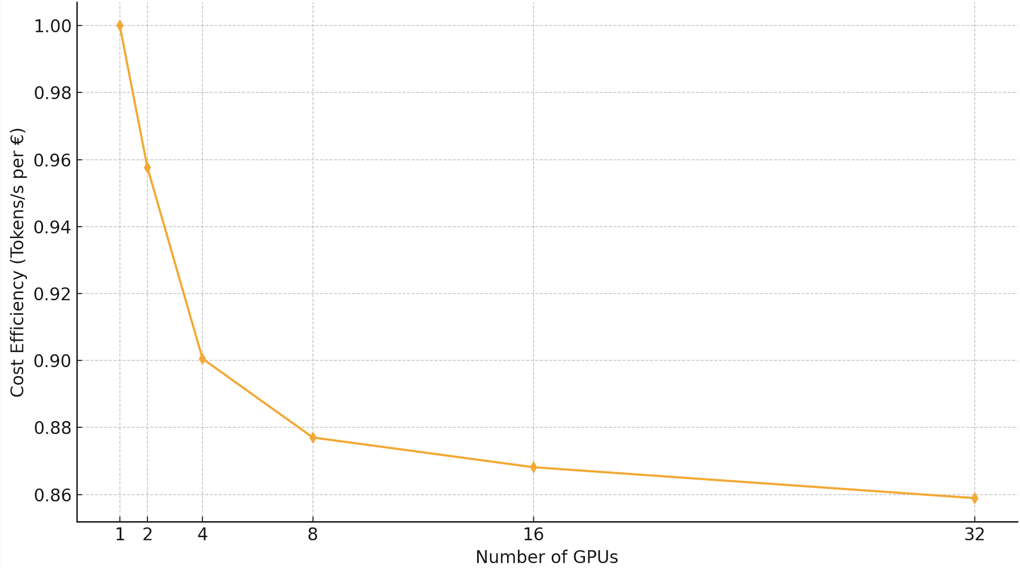
A graph with a line AI-generated content may be incorrect.

Figure 15.1 – Cost-efficiency of training (proxy metric: tokens/s/€). Although total throughput scales, the efficiency per euro slightly declines with more GPUs.

This analysis highlights a key principle in large-scale AI training: faster is not always cheaper. Under tight budgetary or sustainability constraints, moderately parallel configurations can offer the best compromise between time-to-solution and economic efficiency.

An important observation is that the same scaling results can justify very different decisions depending on the training objective. The performance curves shown in Tables 15.10–15.12 do not prescribe a single “optimal” GPU count; instead, they provide a quantitative basis for purpose-driven choices.

If the primary goal is to minimize wall-clock time, using the largest feasible number of GPUs may be justified despite the loss in efficiency. If, instead, the goal is to maximize throughput per euro or to operate under a fixed computational budget, configurations with fewer GPUs may be preferable. The data remains unchanged, but the decision varies with the purpose.

In practice, different training scenarios naturally favor different scaling choices. During early experimentation or hyperparameter exploration, smaller GPU counts often provide better cost-efficiency and scheduling flexibility. In contrast, final production training runs may prioritize time-to-solution and justify lower efficiency at larger scale.

This reinforces a central lesson of this chapter: scalability is not an absolute goal, but a means to satisfy a specific operational purpose.

Task 15.13 – Cost-Efficiency Analysis for OPT

Using the distributed scaling results obtained for OPT 1.3B in Task 15.11, build the cost-efficiency table equivalent to Table 15.12.

Proceed as follows:

Use the measured total throughput values for 1, 2, 4, 8, 16, and 32 GPUs.

Normalize all values with respect to the single-GPU case.

Compute for each configuration: relative throughput, parallel efficiency, and relative cost efficiency (tokens/s/€).

Present your results in a table analogous to Table 15.12, and compare them with the LLaMA-based cost-efficiency analysis.

Finally, compare the economic scaling behavior of LLaMA and OPT and discuss:

Which model exhibits better cost-efficiency at scale.

Whether the optimal “sweet spot” in number of GPUs shifts between both models.

Task 15.14 – Final Reflections and Cost–Performance Analysis

Summarize and critically analyze your findings from this lab using the following guiding questions. Your discussion should be quantitative whenever possible, supported by the measurements obtained throughout the chapter for both LLaMA 3.2 1B and OPT 1.3B.

What throughput improvement did you achieve in Task 15.9 compared to the original baseline in Task 15.1? Express the improvement as a multiplicative factor.

Which optimization stage produced the largest single performance jump (mixed precision, full bf16 model precision, Flash Attention, or Liger)? Why do you think this optimization was so impactful at the hardware level?

If the budget is strictly limited, which configuration offers the best performance per euro, and why?

Considering performance, cost, and energy efficiency together, which configuration would you choose in a real-world production scenario, and why?

Conclude with your perspective on the importance of performance tuning in LLM training workflows, and reflect on how the insights gained in this lab can be applied to other Transformer-based models.

This chapter has demonstrated the value of progressive, layered optimization—starting from a single GPU and extending to distributed environments. Through careful tuning of model precision, attention kernels, and distributed training settings, we achieved:

4.5× improvement in throughput on a single GPU via software-level optimizations.
27.5× speedup when scaling across 32 GPUs with minimal code changes.
High parallel efficiency (≥86%) thanks to proper batch sizing and use of communication-efficient kernels.
A clear view of cost-efficiency trade-offs, reinforcing the importance of balancing speed with resource constraints.

In large-scale HPC environments, these optimizations translate into faster turnaround, lower energy use, and reduced cost per experiment—making AI research more accessible and sustainable.

Importantly, these performance gains were achieved without modifying the training script itself, thanks to the robustness of PyTorch DDP and Hugging Face’s Trainer class—underscoring how the right software stack simplifies scalable LLM training on HPC systems.

Part V brought together all the foundational elements introduced throughout the book—software environments, hardware-aware optimization, distributed training—to tackle the complexity of training state-of-the-art LLMs. By combining empirical benchmarks with conceptual clarity, we hope this final section enables readers to navigate real-world challenges in AI-scale supercomputing.

Viewed through the lens of the four Foundational Performance Principles introduced throughout the book, this chapter presents a coherent performance narrative. We begin by amortizing overheads and unlocking accelerator efficiency, then exploit hardware-specific capabilities through co-designed kernels and precision modes, ensure that computation and synchronization remain balanced at scale, and finally select the GPU count that best serves the intended objective under cost and energy constraints.

Together, these results illustrate that effective LLM training on supercomputing platforms is not about blindly maximizing scale, but about making informed, purpose-driven decisions grounded in system behavior and economic reality.

Key Takeaways from Chapter 15

Training efficiency is as critical as model accuracy when working with Large Language Models. This chapter emphasized extracting maximumER maximum performance per GPU and achieving efficient scaling across multiple GPUs using modern HPC software stacks.
The chapter started from a transparent and reproducible baseline configuration, progressively applying layered software-level optimizations so that performance gains could be clearly attributed to specific system-level decisions.
Increasing batch size proved effective for amortizing fixed overheads and improving GPU utilization, while rapidly exposing GPU memory capacity as a fundamental limiting factor.
Enabling mixed precision improved computational efficiency and throughput, while revealing that overall memory savings are often constrained by optimizer states and runtime allocations rather than by activations alone.
Switching to full bf16 model precision significantly reduced structural memory pressure and enabled further batch size scaling, at the cost of reduced numerical safety margins that must be managed carefully.
Replacing standard attention mechanisms with Flash Attention (sdpa) delivered a major performance inflection point, drastically reducing memory traffic and shifting execution toward a more compute-efficient regime.
Enabling Triton-based Liger kernels produced the largest single performance gain, yielding a 4.5× throughput improvement over the baseline on a single NVIDIA H100 GPU and enabling batch sizes more than six times larger—when supported by the model architecture.
The final optimized single-GPU configuration achieved over 48,000 tokens/s, compared to approximately 10,500 tokens/s at baseline, demonstrating the impact of hardware-aware, kernel-level optimizations without modifying the Python training code.
Scaling this optimized configuration across up to 32 GPUs using PyTorch Distributed Data Parallel resulted in near-linear total throughput growth, with parallel efficiency remaining above 85%.
As GPU count increased, per-GPU efficiency gradually declined due to communication and synchronization overheads, underscoring the importance of balancing computation and collective communication at scale.
Cost-efficiency analysis showed that faster training is not always cheaper: while large GPU counts minimize wall-clock time, configurations with 4 or 8 GPUs often provide a better trade-off between time-to-solution, cost, and energy consumption.
Taken together, the experiments in this chapter can be interpreted through the lens of the Foundational Performance Principles introduced earlier in the book. The progression from batch size scaling to kernel-level optimization reflects the amortization of fixed overheads; the impact of precision modes, Flash Attention, and Liger kernels highlights the role of hardware–software co-design; the distributed scaling results illustrate the need for balanced computation and communication pipelines; and the cost-efficiency analysis reinforces that scale must ultimately serve a clearly defined purpose.
Overall, this chapter demonstrated the importance of layered, system-aware optimization. Effective large-scale LLM training requires first understanding and optimizing single-GPU performance, and then scaling in a way that aligns with the intended performance, cost, and resource objectives.

This analysis will allow you to assess whether the benefits and limitations of mixed precision generalize across different transformer architectures, even when model sizes are relatively close. ↩