1. Supercomputing Basics

• 1. Supercomputing Basics
  • What is Supercomputing?
    • High Performance Computing vs. Supercomputing
    • Parallelism: The Cornerstone of High Performance Computing
      • Why Parallel Computing?
      • Serial Execution on Standard Computers
      • Parallel Execution in HPC Systems
      • Limitations and Challenges of Parallelization
    • Understanding Parallel Computer Architectures
      • The Von Neumann Model
      • From Single to Multiple Cores
      • Memory Architectures for Parallelism
      • Adding GPUs to the Architecture
    • How Supercomputing Powers Modern Science
      • The Three Paradigms of Science: From Empirical to Simulation
      • Big Data-driven Science (The Fourth Paradigm)
      • AI-driven Science (The Fifth Paradigm)
      • The Evolving Role of the Scientist: The Builder’s Dilemma
    • Barcelona Supercomputing Center and MareNostrum 5
  • Performance in Supercomputing
    • Performance and Metrics
    • Standard Benchmarks in HPC
      • Top500 List
      • Peak Performance vs. Sustained Performance
      • Green500 list
      • Specialized and AI Benchmarks
    • Measuring and Understanding Parallel Performance
      • Speedup
      • Performance Degradation Factors
      • Efficiency
      • Scalability
    • Speedup Bounds and Scalability Models
      • Amdahl’s Law
      • Gustafson-Barsis’s Law
      • Parallel Overhead and the Limits of Speedup Models
  • Key Takeaways from Chapter 1

This chapter provides a conceptual introduction to supercomputing and performance-oriented thinking. It establishes the vocabulary and mental models used throughout the book to reason about parallelism, scalability, and system-level performance.

Readers new to high performance computing (HPC) are encouraged to start here. Readers with prior HPC experience may use this chapter as a refresher or reference, focusing on sections that contextualize modern supercomputing in the era of artificial intelligence.

What is Supercomputing?

Since the advent of artificial intelligence (AI), the field of supercomputing has undergone a significant transformation, rendering some topics traditionally found in supercomputing textbooks less central today, while new areas of focus have emerged.

In this first chapter, we have chosen to retain the classical concepts that form part of the historical foundations and culture of the High Performance Computing (HPC) community, recognizing that understanding these fundamentals remains essential for grasping the field’s evolution. However, throughout the book, we will also introduce the new topics that are increasingly shaping the current landscape of supercomputing, particularly in its application to artificial intelligence.

But what exactly is a supercomputer? In simple terms, a supercomputer is a computing system with capabilities far beyond those of typical general-purpose machines like desktops or laptops. Of course, this definition is somewhat fluid—a laptop today might have outperformed a supercomputer from a few decades ago. Yet, no matter how much consumer technology advances, there will always be a need for even more powerful systems to tackle the most demanding computational challenges.

The origins of supercomputing date back to the 1960s, when Seymour Cray , working at Control Data Corporation, developed the first machines designed specifically for high performance tasks. Since then, supercomputers have become indispensable tools in scientific research and engineering. Today, the global community tracks the evolution of these systems through the Top500 list , an authoritative ranking of the world’s 500 most powerful supercomputers, updated twice a year to reflect the state of the art.

Supercomputers owe their power to parallel computing , a method that enables the simultaneous execution of many operations. Rather than solving tasks one after another, a supercomputer distributes the workload across thousands—or even millions—of processing units, all working together to tackle a complex problem. You can think of it as harnessing the capabilities of countless general-purpose machines focused on the same task at once. This model of computation is at the heart of how modern supercomputers function, and as you progress through this book, you’ll explore the key role that parallelism plays in virtually every aspect of supercomputing.

High Performance Computing vs. Supercomputing

Supercomputing represents one of the most transformative technological advancements of the modern era. Its impact extends across a remarkably diverse range of fields, from the most theoretical sciences to the most immediate practical challenges—such as those posed by artificial intelligence—fundamentally expanding human capabilities and understanding.

Throughout the relatively brief history of computing, no other technological domain has demonstrated a comparable rate of advancement. Early machines of the late 1940s performed fewer than 1,000 operations per second. In contrast, modern supercomputers now routinely exceed 1 exaFLOP—one quintillion floating-point operations per second—with leading systems sustaining performances of approximately 1.7 exaFLOPS. This extraordinary growth has been driven by continuous innovation across hardware technologies, computer architectures, programming models, algorithms, and system software.

While often used interchangeably, high performance computing (HPC) and supercomputing reflect slightly different perspectives—and understanding this distinction helps frame the scope of this book:

• Supercomputing refers specifically to the use of supercomputers—large-scale, specialized computing systems designed to solve problems requiring extreme processing power. It evokes the idea of powerful machines and cutting-edge performance.

• High performance computing, on the other hand, is a broader term. It encompasses not only the hardware (supercomputers themselves) but also the software tools, programming models, resource management techniques, and algorithms that enable performance at scale. HPC represents the field of study and practice that makes supercomputing possible and effective.

In practice—particularly in education—the two terms are often used interchangeably. As an academic, I have traditionally favored the term HPC, which I consistently employed throughout the earlier stages of my career. However, over time, supercomputing has gained broader recognition and resonance, especially among non-specialist audiences and university students. Its clarity and immediate impact often make it the more intuitive choice. For this reason, although we have titled this book with the term supercomputing, throughout its content we will use both terms interchangeably.

At its core, HPC is concerned with achieving the greatest computing capability possible at any given point in time and technology. This means continually pushing the boundaries of what is computationally feasible using the best available hardware and software technologies. It is a dynamic field, constantly adapting to new scientific challenges and emerging computational paradigms. In summary, HPC is a field at the intersection of technology, methodology, and application, integrating all these facets:

• Technology — the physical and architectural design of computing systems, including CPUs, GPUs, memory hierarchies, interconnects, and storage.

• Methodology — the techniques used to parallelize, coordinate, and scale computations across many processing units, nodes, and accelerators.

• Application — the scientific or industrial problems that drive the need for high computing power: from climate modeling and genomics to fluid dynamics.

This convergence makes HPC, especially when combined with advances in AI, a foundational discipline for modern research and technological innovation.

Parallelism: The Cornerstone of High Performance Computing

Why Parallel Computing?

For several decades, improvements in processor performance were primarily driven by increases in clock frequency. From the early 1990s to around 2010, clock speeds rose steadily—from approximately 60 MHz to nearly 5 GHz—allowing software to run faster simply by upgrading to the latest CPU. However, this trend has now stalled due to physical limitations in miniaturization, power consumption, and heat dissipation. As a result, continuing performance gains through faster single-core processors has become increasingly impractical and costly.

Modern computing systems instead pursue performance improvements through parallelism—by using multiple moderately fast processing units working together. This strategy is both more scalable and energy-efficient, and it has become the cornerstone of high performance computing in the post-frequency-scaling era.

Serial Execution on Standard Computers

One of the fundamental principles behind HPC is parallelism —the ability to divide a computational task into smaller parts that can be executed simultaneously across many processing units¹. Parallelism is the key to achieving the high performance levels required to solve complex scientific and engineering problems. It is what transforms a large computational challenge from something intractable into something feasible.

On a standard laptop or desktop computer, most programs are designed to execute serially—that is, instructions are carried out sequentially on a single processing unit². This execution model is generally adequate for everyday computing tasks such as web browsing, word processing, or lightweight programming. While modern laptops can achieve a degree of concurrency by assigning different serial applications to run simultaneously on separate processor units, serial execution quickly becomes a bottleneck when it comes to large-scale simulations, big data processing, or training large deep learning models. The limitations of a single processing unit—in terms of computation speed, memory, and data throughput³—make it impractical or even impossible to process such workloads efficiently.

Parallel Execution in HPC Systems

In contrast to traditional sequential execution, where instructions are processed one after another on a single CPU (see Figure 1.1, top), high performance computing systems are designed to execute tasks in parallel. In a sequential program, a problem is broken down into a list of instructions that are executed in order by a single processor. While this model is simple and sufficient for general-purpose computing, it becomes a severe bottleneck for time-sensitive or large-scale workloads.

As illustrated in Figure 1.1 (bottom), parallel execution enables a problem to be divided into independent sub-tasks, each processed simultaneously on a different CPU or node. This parallelism allows large computations to scale in both speed and memory capacity, enabling scientific and engineering challenges to be tackled effectively.

This model usually involves additional complexity: each sub-task must be assigned to a processor, and synchronization and communication between them may be required. However, the benefits in performance and scalability far outweigh the overhead in many HPC use cases.

There are two primary motivations for using parallelism in HPC:

• To reduce execution time: By distributing a problem across multiple processing units, the total time to solution can be drastically shortened. This is especially important in time-sensitive applications such as weather forecasting or epidemiological simulations, where timely decisions are essential.

• To solve problems that exceed the capabilities of a single machine: Large-scale scientific workloads—such as climate modeling, training of state-of-the-art neural networks, or massive genomic analyses—demand computational and memory resources far beyond what a single system can provide.

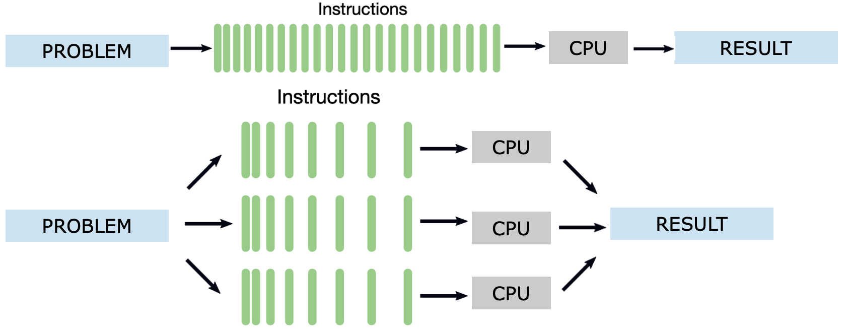
Figure 1.1 – Sequential vs. parallel execution of a computational task. In the sequential model (top), a single stream of instructions is executed by one CPU. In the parallel model (bottom), the problem is divided into parts, each with its own instruction stream executed concurrently on different CPUs, leading to faster and more scalable results.

In addition to task-level parallelism within a single problem, HPC systems are also well-suited for concurrent execution of multiple independent problems. This scenario is common in shared supercomputing environments, where many users or experiments must run simultaneously. As shown in Figure 1.2, each problem is processed independently by a dedicated CPU or core, with its own instruction stream and result. This form of parallelism maximizes resource utilization without requiring communication or synchronization between tasks. It is particularly effective for parameter sweeps, hyperparameter tuning, or serving multiple users in parallel.

This form of parallelism is referred to as concurrency, and it enables efficient utilization of the available computing resources.

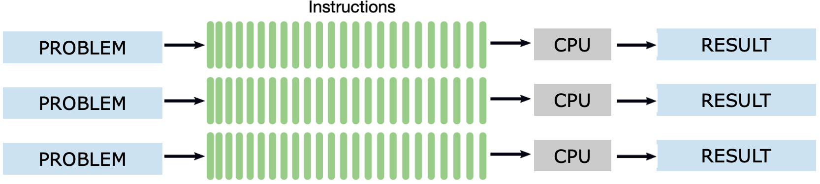
Figure 1.2 – Concurrency through the execution of multiple independent problems. Each problem follows its own instruction stream and is handled by a separate CPU. Unlike parallelism within a single problem (Figure 1.1), concurrency focuses on executing independent computations in parallel, thereby enhancing overall system throughput and efficiency.

Limitations and Challenges of Parallelization

Despite its advantages, not all problems benefit equally from parallel execution. Some programs are inherently sequential or exhibit limited scalability. There are several reasons for this:

• Task dependencies: Some algorithms require the result of one computation before another can proceed. These data or control dependencies introduce delays and force some computations to wait, reducing parallel efficiency.

• Imbalanced workloads: If tasks are not evenly divided, some processors may finish earlier than others and remain idle, resulting in inefficient resource utilization.

• Redundant computations: In certain programs, portions of the code may need to be replicated across tasks when running in parallel. This can add unnecessary overhead, especially when memory usage or data access becomes a bottleneck.

The challenge in HPC is not just to parallelize a problem, but to do so in a way that is efficient, scalable, and sustainable across many nodes. This requires careful algorithmic design and often specialized programming models—many of which will be introduced later in this book.

Understanding Parallel Computer Architectures

Before diving into supercomputing building blocks and programming models for parallel computing, it’s essential to understand how computer architectures have evolved to support parallelism. This includes both historical context—such as the classical Von Neumann architecture—and modern adaptations that incorporate multiple CPUs and GPUs working together in distributed environments. This foundational knowledge will help us better understand the performance characteristics and limitations of parallel applications running on today’s supercomputers.

The Von Neumann Model

The Von Neumann architecture (Figure 1.3), introduced in the 1940s, has served as the conceptual backbone of most modern computing systems. It describes a simple and elegant design in which a single processing unit retrieves and executes instructions sequentially from a shared memory.

In this architecture, the Central Processing Unit (CPU) consists of three main components: the control unit, which orchestrates the execution of instructions; the arithmetic and logic unit (ALU), responsible for basic computations and logical operations; and the registers, which act as the CPU’s fastest memory, holding temporary data for immediate processing.

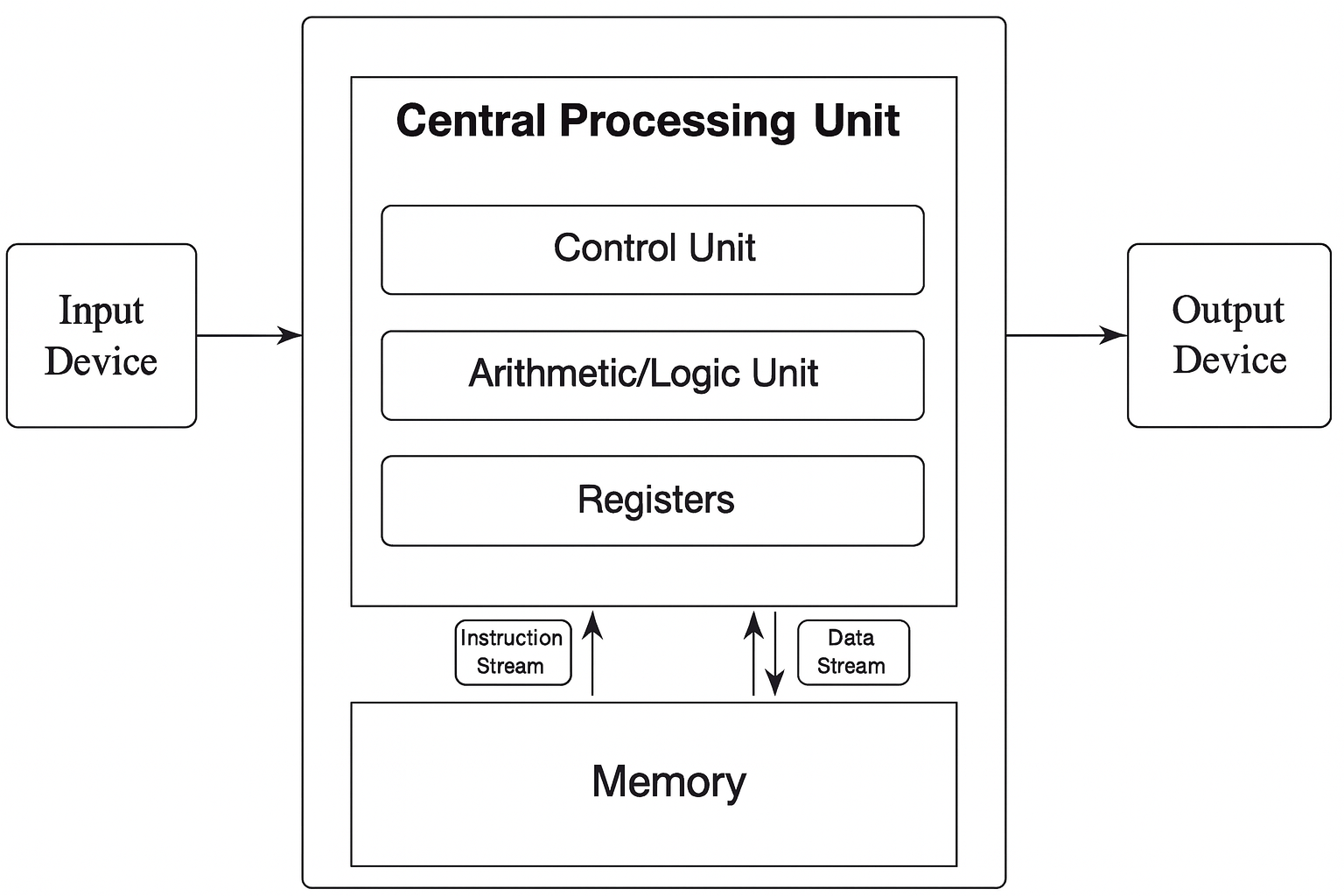
Figure 1.3 – The von Neumann architecture. The CPU contains a control unit, arithmetic/logic unit, and registers. Both instructions and data are stored in the same memory space and accessed sequentially.

This model also includes memory for storing both instructions and data, and input/output devices that interface with the external world. Despite its simplicity, this architecture remains relevant today and provides the foundation for understanding more complex systems.

From Single to Multiple Cores

Over time, computing demands increased beyond what a single processor could handle. To address this, computer chips evolved to include multiple cores, each capable of executing its own instruction stream. Modern CPUs, while still based on the von Neumann model internally, typically integrate several of these cores, each acting as a mini-CPU.

For example, a standard server CPU in 2025 may include 64 cores, enabling it to process multiple tasks in parallel. However, it’s important to distinguish between a “CPU” as a physical package and a “core” as a processing unit inside that package. From a programming perspective, each core can be thought of as an independent processor.

Memory Architectures for Parallelism

The organization of memory plays a crucial role in enabling efficient parallel execution. Two principal models are used in parallel computing systems: shared memory , and distributed memory , each with distinct advantages and challenges.

In shared memory systems, all processors have access to a common memory space (Figure 1.4). This simplifies programming, as all data can be accessed uniformly. However, contention arises when many processors try to access memory simultaneously, which can limit scalability.

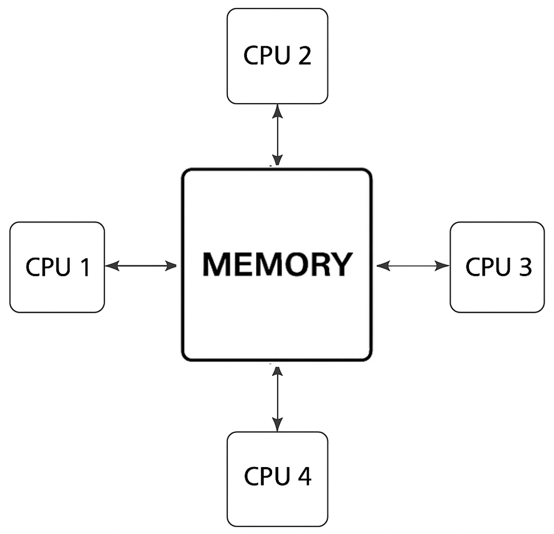
Figure 1.4 – Shared memory (UMA, Uniform Memory Acces). All CPUs access the same memory space with equal latency. Suitable for systems with a limited number of processors.

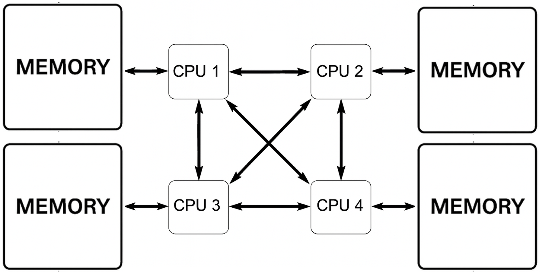
Figure 1.5 – Shared memory (NUMA). Each CPU has faster access to its local memory but can still access remote memory. Improves scalability compared to UMA.

As systems grew larger, the Non-Uniform Memory Access (NUMA) architecture emerged (Figure 1.5). In NUMA systems, each processor accesses its local memory faster than memory attached to other processors. This reduces contention but introduces complexity, as data placement affects performance.

Alternatively, distributed memory systems (Figure 1.6) assign each processor its own private memory. Processors communicate through explicit message-passing over a network. This model scales well and is used in large supercomputers, but it increases programming complexity.

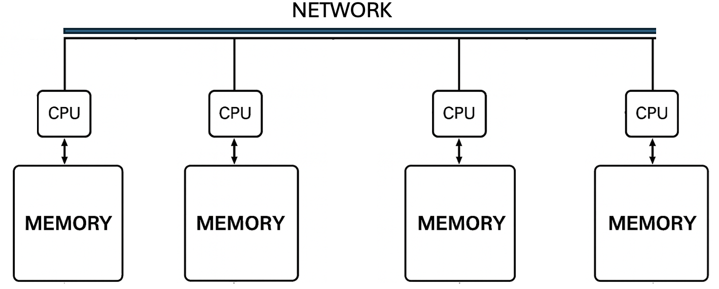
Figure 1.6 – Distributed memory architecture. Each CPU accesses its own local memory and communicates with others via a high-speed network.

To combine the best of both worlds, many HPC systems now adopt hybrid architectures that integrate shared and distributed memory models (Figure 1.7). Within a node, multiple processors may share memory; across nodes, communication occurs over a network. This is the dominant model in supercomputing today.

Adding GPUs to the Architecture

While the architectures described so far focus on CPUs, modern supercomputers heavily rely on Graphics Processing Units (GPUs) to accelerate performance. GPUs are specialized processors originally designed for rendering graphics, but their highly parallel architecture makes them ideal for scientific computing and deep learning.

Each GPU contains thousands of smaller cores optimized for throughput rather than latency. In contrast to CPUs, which are best suited for executing a few complex tasks at high speed, GPUs can simultaneously handle a large number of simple operations. This makes them especially powerful for data-parallel computations found in artificial intelligence and highperformance scientific simulations.

In contemporary HPC systems, GPUs act as co-processors, meaning they do not operate independently but are orchestrated by the CPU, which offloads compute-intensive tasks to the GPU. This collaboration allows the system to leverage the strengths of both architectures—CPUs for control logic and serial execution, and GPUs for high-throughput parallelism.

To support this, each node in a modern supercomputer typically includes multiple CPUs and GPUs, connected via high-speed links. These hybrid nodes are then connected to each other across a high-speed interconnect network, enabling them to work together as a single distributed system while maintaining fast internal communication (Figure 1.8).

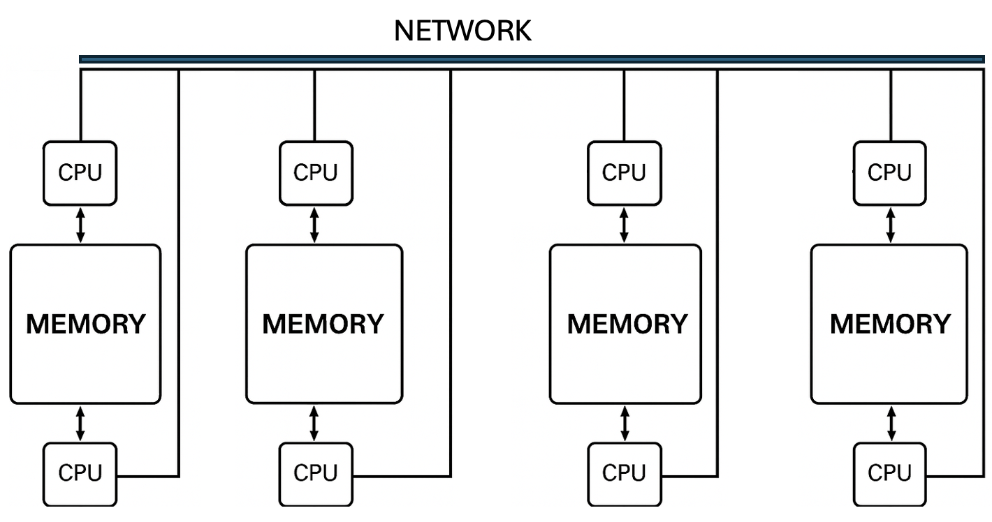
Figure 1.7 – Hybrid distributed-shared memory. Each node contains two CPUs with shared memory; nodes are interconnected via a network. Enables scalable yet flexible parallelism.

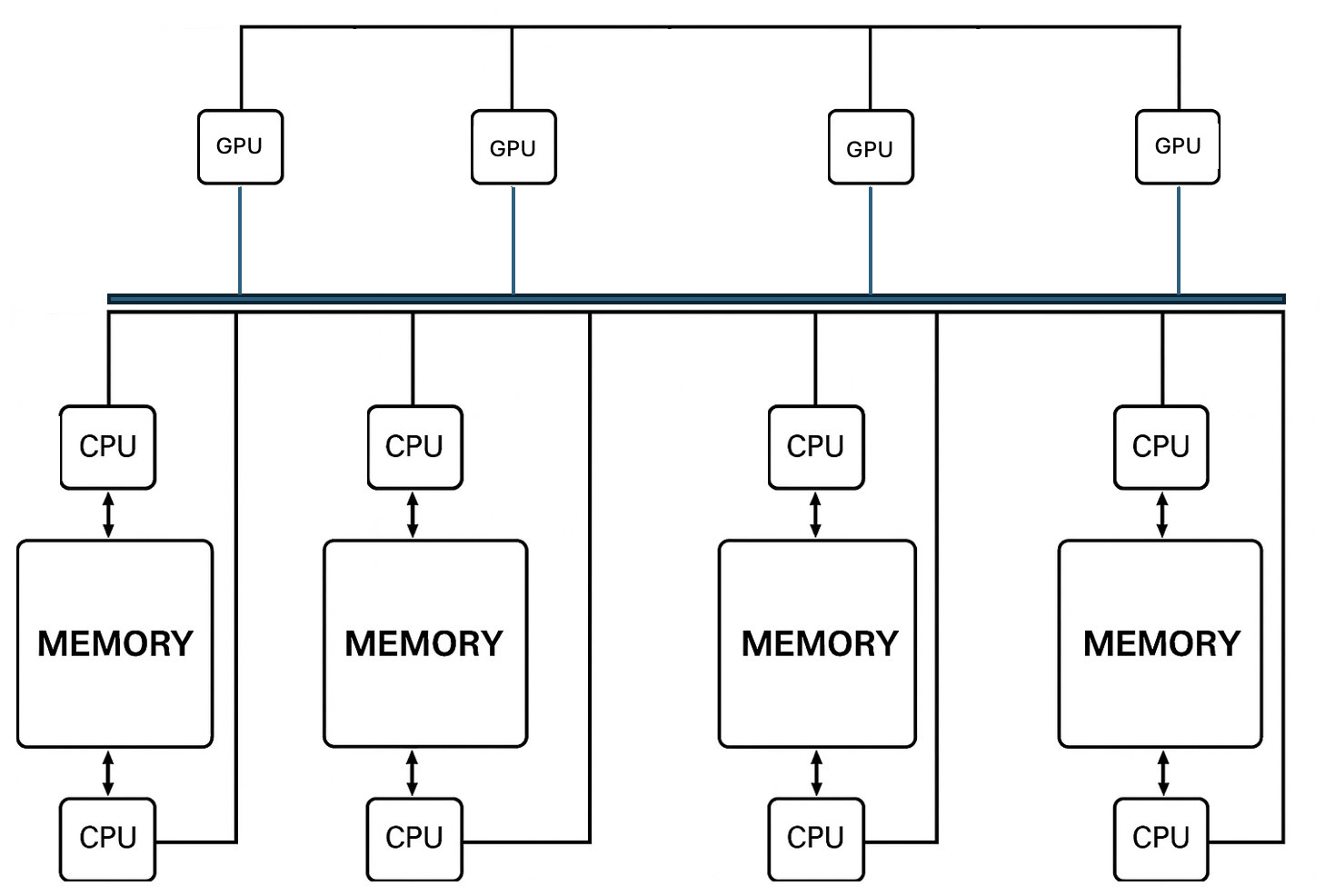
Figure 1.8 – Hybrid CPU-GPU architecture with distributed nodes. Each node combines multiple CPUs and GPUs with local memory. Inter-node communication is enabled via a high-speed network.

This combination of shared memory within nodes and distributed communication across nodes forms the basis of nearly all current supercomputing platforms. In the following chapters, we will explore in greater detail how to program and optimize applications for these hybrid CPU-GPU systems.

How Supercomputing Powers Modern Science

Throughout history, scientific discovery has traditionally rested on two fundamental paradigms: experimentation and theory. For centuries, the cycle of observation, hypothesis formulation, experimentation, and theoretical refinement has provided the foundation for our understanding of the natural world. Classical science advanced through this iterative process, building robust explanations of phenomena based on measurable reality.

However, as the complexity of scientific questions has grown, traditional methods have encountered significant limitations. Some phenomena are too dangerous to test (e.g., nuclear fusion), too expensive to replicate (e.g., jet crash tests), too slow to observe (e.g., climate change), or simply too vast or too small to manipulate physically.

In these situations, an additional tool has become indispensable, leading to the emergence of new paradigms.

The Three Paradigms of Science: From Empirical to Simulation

Following the advent of computers in the mid-20th century, and particularly with the emergence of simulation capabilities —made possible by supercomputers since the 1990s— Computational Science was established as the third paradigm of scientific inquiry, complementing theory and experiment.

This approach allows scientists to create virtual models of reality and test hypotheses computationally, offering insights where direct experimentation is impractical or impossible. Thanks to supercomputing, simulations are often performed before any physical prototype is built or any real-world measurement is taken, through the use of powerful digital twins, which represent the current evolution of numerical simulations. In this paradigm, supercomputers serve as virtual laboratories, enabling new modes of discovery that extend far beyond the reach of classical experimentation.

Big Data-driven Science (The Fourth Paradigm)

With the explosion of data availability at the beginning of this century, spanning fields from genomics to astrophysics, science underwent a fundamental shift.

Instead of explicitly simulating physical laws, researchers began to rely heavily on machine learning, pattern recognition, and anomaly detection to extract meaningful insights from massive datasets. Scientific discovery increasingly involves approximating physical laws from empirical data, an approach particularly effective when dealing with large, complex, or noisy datasets. This fourth paradigm —Big Data-driven Science—  marked a transformative shift in the way scientific discovery is conducted.

AI-driven Science (The Fifth Paradigm)

We are now living in a vibrant moment for science. Building upon the advancements of the Fourth Paradigm, the 21st century has witnessed the emergence of an even more transformative paradigm: AI-driven Science. While the Big Data-Driven Science enabled massive analysis, the Fifth Paradigm takes a crucial step further: AI is leveraged not only to detect patterns but also to actively generate hypotheses and accelerate the discovery process itself.

In this new context, AI is no longer merely an analysis tool; it becomes an autonomous collaborator, proposing new lines of inquiry, designing experiments, and optimizing research strategies. Discovery is becoming not only faster but also increasingly automated and scalable. This progression, from empirical science to autonomous hypothesis generation, is clearly illustrated in Figure 1.9.

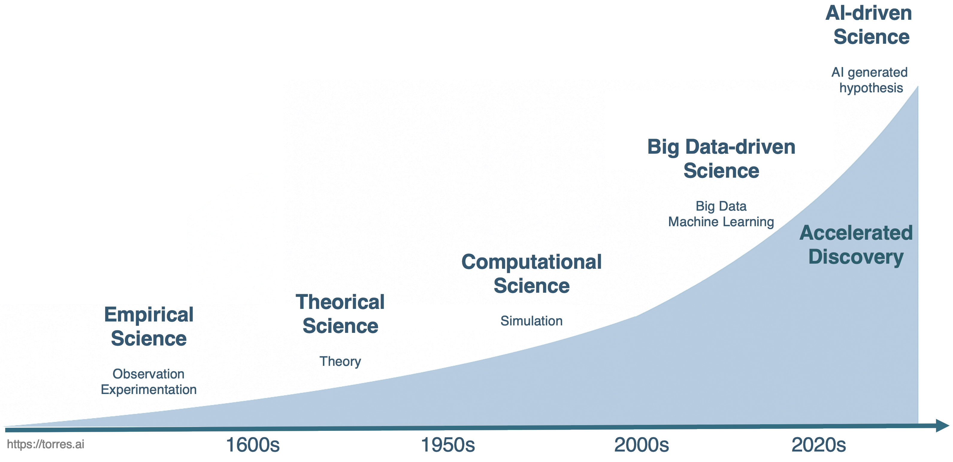
Figure 1.9 – Evolution of scientific paradigms throughout the history of science.

Figure 1.9 illustrates the progression of scientific discovery over time, from empirical science based on observation and experimentation to the current frontier of AI-driven science, which introduces autonomous hypothesis generation and accelerated discovery—achieving breakthroughs in ways previously unimaginable.

The Evolving Role of the Scientist: The Builder’s Dilemma

This acceleration, made possible by modern supercomputing infrastructures capable of training powerful AI models, is changing the very nature of scientific work. The reflection offered by Oriol Vinyals (a key figure behind systems such as AlphaFold and Gemini) in his 2025 acceptance speech for an honorary doctorate from the Universitat Politècnica de Catalunya, is particularly insightful.

Vinyals frames this transformation not primarily in terms of speed or computational power, but in terms of how the role of the scientist is evolving.

One of his central ideas is simple yet deeply consequential: in a world where AI can execute experiments and analyze data, the true value of the scientist increasingly lies in asking the right questions. When machines can explore hypotheses at a scale no human could match, formulating meaningful, well-posed scientific questions becomes not just important, but essential.

This shift leads to what Vinyals calls the “builder’s dilemma”: the uneasy feeling that, by creating systems capable of scientific reasoning, we might be designing tools that eventually perform our own work better than we do. However, he proposes a different interpretation: AI should be understood as an amplifier of human curiosity and creativity, not as its replacement. It is a tool that expands what we can explore, not one that eliminates the need for human insight.

The scientist’s role moves away from executing every experiment toward orchestrating exploration through questions. Supercomputing provides the physical infrastructure that makes this transformation possible; AI provides the cognitive machinery that reshapes discovery. But neither replaces the need for scientific judgment, ethical responsibility, and intellectual curiosity.

Vinyals closes his reflection with a message that is both sobering and hopeful: technologies will continue to change at an accelerating pace, but curiosity, critical thinking, and the ability to ask good questions will remain the most valuable scientific skills. The challenge for the next generation of scientists and engineers will not be to compete with machines at what they do best—but to learn how to guide them toward meaningful discovery.

Barcelona Supercomputing Center and MareNostrum 5

The Barcelona Supercomputing Center–Centro Nacional de Supercomputación (BSC) is Spain’s national supercomputing facility and a recognized leader in HPC in Europe. It manages MareNostrum 5 supercomputer and provides advanced computational resources to both the international scientific community and industry. Its research activity spans five main areas: Computer Sciences, Life Sciences, Earth Sciences, Engineering Applications, and Computational Social Sciences.

BSC coordinates the Spanish Supercomputing Network (RES), was a founding member of the former European infrastructure PRACE (Partnership for Advanced Computing in Europe), and currently serves as a hosting entity of EuroHPC JU, the Joint Undertaking that leads large-scale supercomputing investments at the European level. The center plays an active role in major European HPC initiatives and maintains close collaboration with other top-tier supercomputing institutions across Europe.

The MareNostrum 5 (MN5) machine, housed at the BSC premises in Barcelona, is of particular importance to this book. Since our practical exercises will utilize the MN5 infrastructure, its presence underpins many of the concepts discussed in the following chapters.

MN5 is designed to support the development of next-generation applications, including those leveraging AI, providing the massive scale and low-latency needed for the AI-driven science paradigm (as discussed in the previous section).

BSC inherits the legacy of the European Center for Parallelism of Barcelona (CEPBA), a pioneering research, development, and innovation center in parallel computing technologies. CEPBA was established at the Universitat Politècnica de Catalunya (UPC) in 1991, consolidating the expertise and needs of several UPC departments, particularly the Department of Computer Architecture.

In 2000, CEPBA entered into a collaboration agreement with IBM to create the CEPBA-IBM Research Institute, which paved the way for the formal establishment of the BSC in 2005, with an initial team of 67 staff members. Today, BSC employs more than 1,400 professionals, including over 1,100 researchers—a distinctive feature that sets it apart from other supercomputing centers worldwide: the strong integration of cutting-edge research and HPC infrastructure under the same institution.

Performance in Supercomputing

Performance and Metrics

Understanding the performance of a supercomputer is essential for evaluating its capabilities, yet this concept, while seemingly intuitive, is far from simple. No single measurement can fully capture all aspects of a supercomputer’s operational quality. Instead, multiple quantifiable parameters — known as metrics — are routinely applied to characterize the behavior and efficiency of HPC systems. A metric in supercomputing is defined as an observable and quantifiable operational parameter that provides insight into how a system performs under specified conditions.

At the foundation of performance measurement lie two fundamental dimensions: the amount of time required to complete a given task, and the number of operations performed during that task. These two measures are often combined to create practical evaluation standards. Among them, the most widely used metric is FLOPS — Floating-Point Operations Per Second — which measures how many arithmetic operations (specifically, addition or multiplication of real numbers) a system can perform in one second. FLOPS provides a standardized, hardware-independent way to compare the raw computational capabilities of different supercomputers.

Throughout this book, we adopt the FLOPS notation (e.g., PFLOPS, EFLOPS) to express floating-point performance. However, readers may encounter alternative notations in the literature, such as PFlop/s or simply flops (in lowercase), all referring to the same concept: the number of floating-point operations per second. While the capitalization may vary, the underlying unit remains consistent.

In essence, FLOPS is a measure of throughput—a key performance concept that describes the rate at which a system processes work over time. In the context of HPC, throughput refers to the number of useful operations completed per unit of time, reflecting how effectively a supercomputer utilizes its computational resources. We will return to this concept later in the book, when we explore the different types of throughput used in various contexts.

Given the extraordinary scale of performance in modern computing, it is necessary to use scientific prefixes to express these large numbers compactly: kilo (10³), mega (10⁶), giga (10⁹), tera (10¹²), peta (10¹⁵), and exa (10¹⁸).

For example, early supercomputers achieved performance levels around 1 kiloFLOPS (10³ FLOPS), while today’s leading systems surpass the exaFLOP barrier, routinely achieving performances on the order of 10¹⁸ FLOPS. Meanwhile, modern laptops, which have seen remarkable growth in their own right, can reach several teraFLOPS (10¹² FLOPS), showing that while personal computing power has grown dramatically, it still lags millions of times behind top-tier supercomputers when measured by raw FLOPS. .

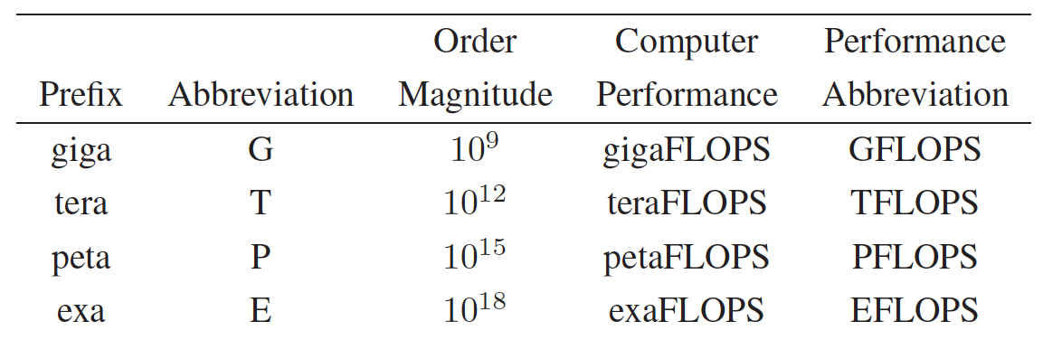
Table 1.1 – Scientific prefixes commonly used to express computer performance in FLOPS.

Standard Benchmarks in HPC

While FLOPS is a widely used metric for quantifying computational capacity, it has inherent limitations. FLOPS measures the potential arithmetic throughput of a system, but not how efficiently real-world applications are executed—especially those constrained by memory bandwidth, I/O bottlenecks, or algorithmic complexity. To address this gap, the HPC community relies on standardized benchmark applications that simulate realistic workloads. These benchmarks allow for meaningful comparisons between systems by measuring the time required to complete well-defined computational tasks under controlled conditions..

Top500 List

One of the most prominent benchmarks in HPC is the Highly Parallel Linpack (HPL). HPL evaluates how efficiently a system can solve large, dense systems of linear equations using floating-point arithmetic, and it forms the basis of the Top500 list⁴—a biannual ranking of the world’s 500 most powerful supercomputers.

Although HPL does not represent the full diversity of scientific workloads, it provides a consistent and historically rich measure of system capability. Figure 1.10 illustrates the exponential growth in supercomputing performance over recent decades, based on HPL data reported in the Top500 list. The plot shows the combined performance of all ranked systems, the top-performing system, and the system ranked 500th, highlighting the rapid pace of architectural and computational advances.

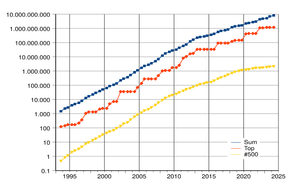
Figure 1.10 – Rapid growth of supercomputer performance, based on data from the Top500 list, adapted from Wikipedia. The logarithmic y-axis shows performance in FLOPS. Top line: Combined performance of the 500 largest supercomputers. Middle line: Fastest supercomputer. Bottom line: Supercomputer ranked 500th in the list (Source: top500.org).

Since its first edition in 1993, the Top500 list ranking has served as a key indicator of progress in HPC, capturing not only performance evolution but also trends in architecture (e.g., the increasing use of accelerators like GPUs), software stack complexity, or the geographical distribution of HPC leadership.

As of the latest edition of the Top500 list, released in November 2025, the El Capitan system at Lawrence Livermore National Laboratory (USA) remains at the top, having achieved 1.8 exaFLOPS on the HPL benchmark. With Frontier(1.3 exaFLOPS) and Aurora (1.012 exaFLOPS) occupying the second and third positions respectively, the Top500 list continues to feature three fully operational exascale systems from U.S. Department of Energy facilities.

A significant highlight of this edition is the formal entry and rise of European systems. Europe’s progress toward exascale is now consolidated by the JUPITER system at Forschungszentrum Jülich (Germany), which fully enters the list at rank four with a confirmed HPL score of 1 exaFLOPS. This achievement marks Europe’s first operational exascale system and represents a crucial milestone in global HPC leadership. Furthermore, the list notes the continued strong presence of cloud-based HPC solutions such as Microsoft Azure’s Eagle (561 petaFLOPS, rank five).

MareNostrum 5 appears in the list under its two major partitions (applications typically run on one partition or the other, not across both simultaneously). The Accelerated Partition (ACC), equipped with NVIDIA H100 GPUs ranks 14th with 175.3 petaFLOPS. The general purpose partition (GPP), based solely on CPUs, remains a vital resource, ranking 50th with 40.1 petaFLOPS. This dual configuration reflects the growing trend in modern supercomputers of combining CPU-only and GPU-accelerated resources to serve a diverse range of scientific and AI workloads.

Peak Performance vs. Sustained Performance

As previously discussed, the Top500 list reports two different performance figures for each supercomputer: Rpeak and Rmax.

• Rpeak, known as peak performance, corresponds to the theoretical maximum number of floating-point operations per second (FLOPS) a system could achieve under ideal conditions if all components were fully utilized without any inefficiencies. Essentially, it reflects the hardware potential of the system based on its architectural specifications.

• Rmax, also called maximum performance, is measured using the HPL benchmark and accounts for various practical factors that affect real execution, such as memory access latency, communication overhead, and Input/Output constraints. It represents the actual number of floating-point operations the system completes during the benchmark, divided by the total wall-clock time.

This dual reporting allows analysts and users to assess both the architectural potential (Rpeak) and how efficiently that potential is realized in practice (Rmax). The official ranking position in the Top500 list is determined by Rmax rather than Rpeak, since it provides a more realistic measure of the system’s usable performance.

While some authors refer to Rmax as a form of sustained performance, it is important to emphasize that running a benchmark is not the same as running real-world applications. Actual workloads may present highly diverse computational patterns, irregular communication patterns, or more demanding I/O requirements, and therefore may not fully exploit the system’s theoretical or even benchmarked capabilities. This is something we routinely observe in real production environments such as MareNostrum 5 at BSC, where application performance often varies significantly depending on the specific workload characteristics.

That said, for the purposes of this book, we will not dwell excessively on these nuances, but it is important for students to be aware that passing the HPL benchmark “exam” with excellent results does not necessarily guarantee equally high performance for all types of real applications.

Moreover, in modern supercomputing, performance alone is no longer sufficient. Energy efficiency has become a key factor: supercomputers must deliver high FLOPS while minimizing power consumption. This growing concern has led to the creation of the Green500 ranking, which highlights the most energy-efficient systems based on FLOPS-per-watt metrics.

Green500 list

As energy consumption and sustainability have become increasingly critical concerns in HPC, evaluating supercomputers based solely on their raw computational performance is no longer sufficient. While the Top500 list ranks systems according to their Rmax values — that is, the maximum sustained floating-point performance measured by the HPL benchmark — energy efficiency has emerged as a parallel and equally important dimension of system evaluation.

To address this, the HPC community introduced the Green500 list as a complementary ranking that highlights the energy efficiency of supercomputing systems. Importantly, Green500 list is not based on a separate benchmark but is directly derived from the same data collected for the Top500. Each system’s energy efficiency is computed simply by dividing its measured Rmax (in FLOPS) by the electrical power consumed during the benchmark run (in watts), resulting in a value expressed in FLOPS per watt.

Since both Rmax and power consumption (reported in kilowatts) are already collected for all Top500 submissions, the Green500 list is automatically generated using this straightforward ratio.

This simple yet meaningful calculation highlights the importance of balancing computational performance with power efficiency. As modern supercomputers continue to scale towards exascale levels, power consumption becomes one of the most significant challenges — both in terms of operational costs and environmental sustainability. Energy-efficient system design now influences nearly every aspect of HPC architecture, including processors, accelerators, interconnects, memory hierarchies, cooling infrastructures, and facility design.

A key observation is that high performance and high energy efficiency are not mutually exclusive. Many of the leading systems on the Green500 list also rank among the most powerful machines on the Top500, demonstrating that cutting-edge performance can be achieved while maintaining responsible power usage. In fact, achieving exascale computing within practical power budgets has driven much of the recent innovation in heterogeneous architectures combining CPUs and GPUs, along with sophisticated power management and optimized cooling technologies (as will be discussed in the next chapter).

Specialized and AI Benchmarks

While both the Top500 and Green500 lists primarily rely on results from the HPL benchmark, it is critical to recognize that no single metric fully captures the complexity of real-world supercomputing workloads. To obtain a multi-dimensional view of system behavior, two categories of complementary benchmarks have emerged: those targeting specific HPC bottlenecks, and those targeting the rising demands of Artificial Intelligence.

1. HPC Workload Benchmarks

These focus on specific performance aspects that HPL does not address:

• HPCG (High Performance Conjugate Gradient): Aims to represent the memory access patterns and communication bottlenecks common in many scientific applications, offering a more representative view of real-world sustained performance.

• STREAM: Measures sustainable memory bandwidth, which is often a limiting factor in data-intensive computations.

• Graph500: Evaluates performance for workloads involving irregular data structures and non-linear memory access, such as those used in graph analytics, sparse matrix operations, and emerging AI workloads.

2. The AI Performance Standard: MLPerf

With the ascendancy of the “AI-driven Science” paradigm, a new standard has become essential for measuring the performance of systems specifically for Machine Learning (ML) workloads.

MLPerf is the industry-standard benchmark suite for measuring the efficiency and speed of AI hardware and software. It is the de facto equivalent of HPL for Artificial Intelligence, designed to evaluate the capability of systems across the entire AI lifecycle.

Although MLPerf provides metrics for AI performance, its deep-dive analysis and practical usage extend beyond the scope required for the purposes of this book. It is, however, an indispensable reference for understanding the current competitive landscape of HPC, where the metric of success is increasingly defined by the ability to handle both traditional scientific simulations and cutting-edge AI workloads.

Taken together, these complementary benchmarks provide a multi-dimensional view of supercomputing capabilities, better reflecting the diverse range of scientific, industrial, and AI workloads encountered in modern HPC facilities and future AI factories.

Measuring and Understanding Parallel Performance

In the HPC community, we typically use the execution time of a program—also known as wall clock time—defined as the elapsed time from when the first processing unit starts execution until the last one finishes, as the basis for constructing various metrics used to compare different parallelization strategies.

The baseline for performance measurement is the time taken by the best serial algorithm to execute the task on a single processing unit, denoted as T_s (serial time). The time taken for the parallel execution of the same task using P processors is denoted as T_P (parallel time).

It is crucial to understand that the parallel execution time (T_P) is not solely composed of computation. In any real-world parallel system, T_P must account for various non-computational costs, collectively known as Parallel Overhead.

Formally, the total execution time on P processors can be modeled as:

T_p = T_comp + T_overhead

Where T_comp is the actual time spent on useful computation, and T_overhead represents the time lost due to parallelization costs. The primary goal of parallel programming is to minimize T_overhead so that the benefits of dividing T_comp by P are maximized.

Speedup

The first and most commonly used metric to quantify the benefit of parallelization is speedup(P). In the supercomputing community we define the speedup as the ratio between execution time in a base configuration (serial time) and the execution in $P$ parallel processing unit:

speedup(P) = T_s ⁄ T_p

In parallel computing, the goal is to equally divide the work among the available parallel processing units in the system while introducing no additional work at the same time. Assume that we run our program with $P$ processing units, then ideally, our parallel program will run P times faster than the serial program. Ideally

speedup(P) = P

In this case, we say that our parallel program has a linear speedup, achieving a one-to-one improvement in performance for each additional processing unit.

However, code or hardware characteristics sometimes will limit the maximum speedup even though we increase the processing units available. The next example will illustrate this situation.

Suppose that we are able to parallelize 90% of a serial program and the speedup of the parallel part is linear regardless of the number of processing units p we use. If the serial run-time T_s is 20 seconds, then the run-time of the parallelized part will be 0.9 * T_s / p = 18 / p and the run-time of the unparalleled part will be 0.1 * T_s = 2. Therefore the overall parallel run-time of this parallel program will be Tp = 18 / p + 2. Finally, the speedup can be defined as Speedup = 20 / (18 / p + 2).

If p gets larger and larger, 18 / p gets closer and closer to 0, so the denominator of the speedup can’t be smaller than 2. Thus speedup will always be smaller than 10.

This illustrates that even if we have perfectly parallelized 90% of the program, and even if we have the whole MareNostrum 5 supercomputer to run this code, we will never get a speedup better than 10.

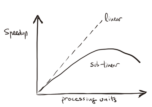
Figure 1.11 – Illustration of sub-linear speedup behavior resulting from performance degradation factors.

On the other hand, serial programs will not have these performance degradation. Thus, it will be very unusual for us to find that our parallel programs get a linear speedup. Furthermore, it is likely that the performance degradation will increase as we increase the number of processing units. Generally as p increases, we expect that the speedup becomes a smaller and smaller fraction of the ideal linear speedup p. We refer to this case as sub-linear speedup (Figure 1.11), normally due to different performance degradation factors. In the next section we will return to this topic of speedup limits.

Performance Degradation Factors

We previously introduced T_overhead as a simplified way to represent the time lost due to parallelization costs and to illustrate performance degradation. In practice, however, this overhead does not originate from a single source, but rather from a complex interplay of multiple factors. The application code written by users, the efficiency of compiler translations, the behavior of the operating system, and the design of the underlying system architecture all contribute to this performance gap. Understanding the causes of degradation is essential for developing strategies that minimize their impact and maximize the effective use of computing resources. Several situations explain why performance is degraded:

• Starvation: Starvation occurs when there is not enough parallel work available to keep all computational resources busy. In a perfectly efficient system, all functional units would operate simultaneously, executing independent instructions every clock cycle. However, if an application lacks sufficient parallelism, or if work is unevenly distributed among processors (load imbalance), some computational units remain idle. This absence of work reduces the overall throughput, leading to lower sustained performance. Addressing starvation often requires improving the parallel structure of the application and ensuring an even load distribution across resources.

• Latency: Latency refers to the delay incurred when data must travel between different parts of the system. When an execution unit must wait for data from a remote location—be it memory, or across nodes—the unit is effectively stalled until the data arrives. High latency can significantly hinder performance by introducing periods of inactivity. Mitigating the effects of latency involves improving data locality (keeping frequently accessed data close to where it is needed) and leveraging hardware features like cache hierarchies and multithreading to “hide” waiting times by overlapping computation with data transfer.

• Overhead: Overhead encompasses all additional work that does not directly contribute to the primary computation but is necessary for managing system resources. Examples include synchronization of parallel tasks, communication setup, or memory management. Although necessary, overhead consumes processing time and hardware resources, reducing the system’s effective throughput. Moreover, high overhead limits how finely tasks can be subdivided, thus indirectly restricting the performance of parallel programs. Reducing overhead through optimized algorithms and runtime systems is critical to improving overall system performance.

• Contention: Contention occurs when multiple threads or processes attempt to access the same resource simultaneously, such as a memory bank or network link. Since only one access can proceed at a time, others must wait, causing delays that extend the execution time of operations. This not only wastes time but also temporarily blocks the associated hardware, leading to inefficient use of computational capacity and increased energy consumption. Furthermore, contention introduces unpredictability into program execution, making performance optimization more challenging.

Ultimately, real-world performance is shaped by the cumulative impact of these factors, each contributing to a gap between observed performance and the theoretical peak. Mastering the effective design and use of supercomputing systems therefore requires a deep understanding of the mechanisms that lead to performance degradation, as well as proactive strategies to mitigate their effects.

These concepts will reappear throughout this book in different contexts and at different levels of detail. When referring to parallel performance degradation in a general and abstract manner, without analyzing its specific causes, we will use the term overhead.

Efficiency

In order to measure the percentage of ideal performance is achieved, we define a new metric, the efficiency of a parallel program (or parallel efficiency), as

efficiency(P) = speedup(P) ⁄ P

Given this definition, we expect that 0 ≤ Efficiency ≤ 1 and it is giving us a measure of the quality of the parallelization process. If efficiency is equal to 1, this means that the speedup is P, and the workload is equally divided between the P processing units which are utilized 100% of the time (linear speedup).

Let’s revisit the previous scenario, where a parallelized program has a Speedup(P) = 10 when using P = 32 processing units. According to the definition of efficiency:

efficiency(32) = speedup(32) ⁄ 32= 10/32 = 0.3125

This means that each processor is being used at only 31.25% of its ideal capacity. The efficiency is far from perfect, even though we achieved a significant speedup.

It is clear that T_P, speedup, and efficiency depend on P, the number of processing units, but also all depend on the problem size. We will return to this topic later.

Finally, mention that there are situations wherespeedup(P) > P* and efficiency(P) > 1 in what is known as super-linear speedup. In Figure 1.12 we represent this situation. According to the interpretation we gave to efficiency, this seems like an impossible case, but taking timing from programs (as we will introduce later), we can find this case.

A parallel system might exhibit such behavior if its memory is hierarchical and if access time increases (in discrete steps) with the memory used by the program. In this case, the effective computation speed of a large program could be slower on a serial processing element than on a parallel computer using similar processing elements. This is because a sequential algorithm using M bytes of memory will use only M/P bytes on each processor of a P processing units on a parallel computer and for instance the working set of a problem is bigger than the cache size when executed sequentially, but can fit nicely in each available cache when executed in parallel. This situation can come from vast amount of places as cache usage, memory hit patterns (divides problem differently than in sequential application). Cache and virtual memory effects could reduce the serial processor’s effective computation rate.

Other reasons for super-linear speedup are simply better (or a slightly different) parallel algorithm or different compilation optimizations, etc.

Task 1.1 – Playing with Speedup and Efficiency

Imagine a parallel program that runs in 100 seconds on a single processing units. When executed on 10 processors, it completes in 15 seconds. Compute the speedup achieved when using 10 processors and the corresponding efficiency.

Reflect: Is the speedup linear? Why or why not? What could explain the observed efficiency?

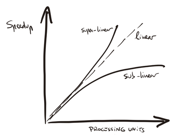
Figure 1.12 – Super-linear speedup vs sub-linear speedup.

Scalability

In the HPC community, we say that a system is scalable if it preserves high efficiency even as more computational resources are added.

Two main types of scalability are typically distinguished in HPC:

• Strong scalability: A program is said to be strongly scalable if its efficiency remains stable as the number of processing units increases, without changing the problem size. In this case, the program should ideally take 1/P of the time to compute the result when using P processing units.

• Weak scalability: A program is weakly scalable if its efficiency remains stable when both the number of processors and the problem size increase proportionally. This means the program takes approximately the same time to solve a problem that is P times larger using P times more resources.

In other words, weak scalability refers to scenarios where the problem size increases proportionally with the number of processing units, with the objective of maintaining a constant execution time. In contrast, strong scalability refers to scenarios where the problem size remains fixed while the number of processing units increases, aiming to reduce execution time proportionally.

To illustrate strong scaling, suppose a program takes 120 seconds to run on 1 processor. When executed on 8 processors, the execution time drops to 18 seconds. This gives a speed-up of 120/18 ≈ 6.7, compared to the ideal of 8, and an efficiency of approximately 84%. The significant reduction in runtime, despite falling short of perfect efficiency, indicates good strong scalability as the workload remains fixed while resources increase.

Now consider weak scaling. If each processor handles 1 million cells, the problem size increases proportionally with the number of processors. With 1 processor (1M cells), the program takes 120 seconds. When run on 8 processors (8M cells), it completes in 135 seconds. Since the runtime increases only slightly, the weak scaling efficiency is 120/135 ≈ 0.89, or 89%. This suggests that the program maintains reasonable performance even as both workload and resources scale up together.

In simple terms, strong scalability reflects how adding more processors makes the program faster for the same problem (i.e., speedup with fixed problem size), while weak scalability indicates whether the program can handle larger problems without increasing runtime as more processors are added (i.e., constant runtime with proportionally increasing problem size).

Task 1.2 – Understanding Strong and Weak Scaling

To deepen your intuition about scalability, consider the following thought experiment. Suppose you are analyzing the performance of a parallel program under two different execution strategies. In the first case, you want to solve a fixed-size problem faster by using more processors. You run the same workload on 1, 2, 4, 8, and 16 processors and observe the following execution times: 120, 70, 40, 28, and 25 seconds, respectively. In the second case, you scale the problem size proportionally to the number of processors so that each processor always receives the same amount of work. With this setup, the program takes 120 seconds on 1 processor, 125 seconds on 2 processors, 132 seconds on 4 processors, 140 seconds on 8 processors, and 160 seconds on 16 processors.

Reflect on how these two situations illustrate the concepts of strong scaling and weak scaling. For the fixed-size case, try to estimate the speedup and efficiency at each processor count. Then, observe when the benefits begin to diminish and speculate why that might occur. For the scaled-size case, consider whether the increase in total runtime is acceptable and what factors could explain the degradation, even if each processor is doing the same amount of work.

Use these scenarios to articulate in your own words the practical difference between strong and weak scaling.

Since scaling is a term that we frequently use in the HPC community, often appearing in the middle of any technical discussion, it is worth taking a closer look at its implications.

Is strong scaling always better?

Strong scaling is more demanding because it requires reducing the execution time of a fixed-size problem as more resources are added. It is ideal for problems where the problem size is fixed (e.g., real-time systems, strict deadlines, or simulations with fixed resolution).

Weak scaling, on the other hand, is often more realistic for problems where the problem size can grow along with the available resources (e.g., climate simulations, hyperparameter searches, or training large language models with increasing datasets).

In real scientific workloads running on systems like MareNostrum 5, many codes are designed to achieve good weak scalability, as the goal is often to utilize larger machines to solve larger problems.

Therefore, while strong scaling is desirable when achievable, it is not always applicable or necessarily better.

Does good strong scaling imply good weak scaling and viceversa?

However, in practice, this is often not the case. Some workloads scale well in weak scaling (i.e. because computation grows faster than communication), but not in strong scaling (i.e. because dividing the problem into smaller chunks can reduce per-task efficiency). Communication latencies, memory access contention, synchronization overheads, and algorithmic complexities often lead to different bottlenecks in weak versus strong scaling. Furthermore, many algorithms exhibit overheads that increase with problem size.

In summary, both forms of scalability address different scenarios and are subject to distinct performance limitations.

Speedup Bounds and Scalability Models

To gain an intuitive understanding of the theoretical limits of speedup in parallel computing, we often refer to two of the most classical and widely cited models in the HPC field: Amdahl’s Law and Gustafson-Barsis’s Law.

Amdahl’s Law

Amdahl’s Law s probably the most well-known law when discussing parallel systems. In 1967, Gene Amdahl formulated a simple thought experiment to derive the performance benefits that could be expected from a parallel program. Amdahl’s Law provides the theoretical speedup achievable by a system as the number of processing units increases. When Gene Amdahl proposed his law, he could not have foreseen the rapid advances in computer architecture and microelectronics that would lead to single-chip multiprocessors with dozens of processor cores. However, he made a visionary observation that remains highly relevant today: any effort invested in improving parallel processing performance is ultimately limited — and may even be wasted — unless it is accompanied by comparable improvements in sequential processing performance.

Let f be the fraction of operations in a computation that must be performed sequentially, where 0 ≤ f ≤ 1. The maximum speedup achieved by the parallel computer with p processing units performing the computation is

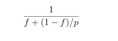
Amdahl’s Law assumes that our goal is to solve a problem of fixed size as quickly as possible. It provides an upper bound on the speedup achievable when applying multiple processing units to execute the problem in parallel. The speedup is fundamentally limited by the fraction of work that cannot be parallelized — the serial portion — which remains constant regardless of the number of processors used (see Figure 1.13 for a visual illustration).

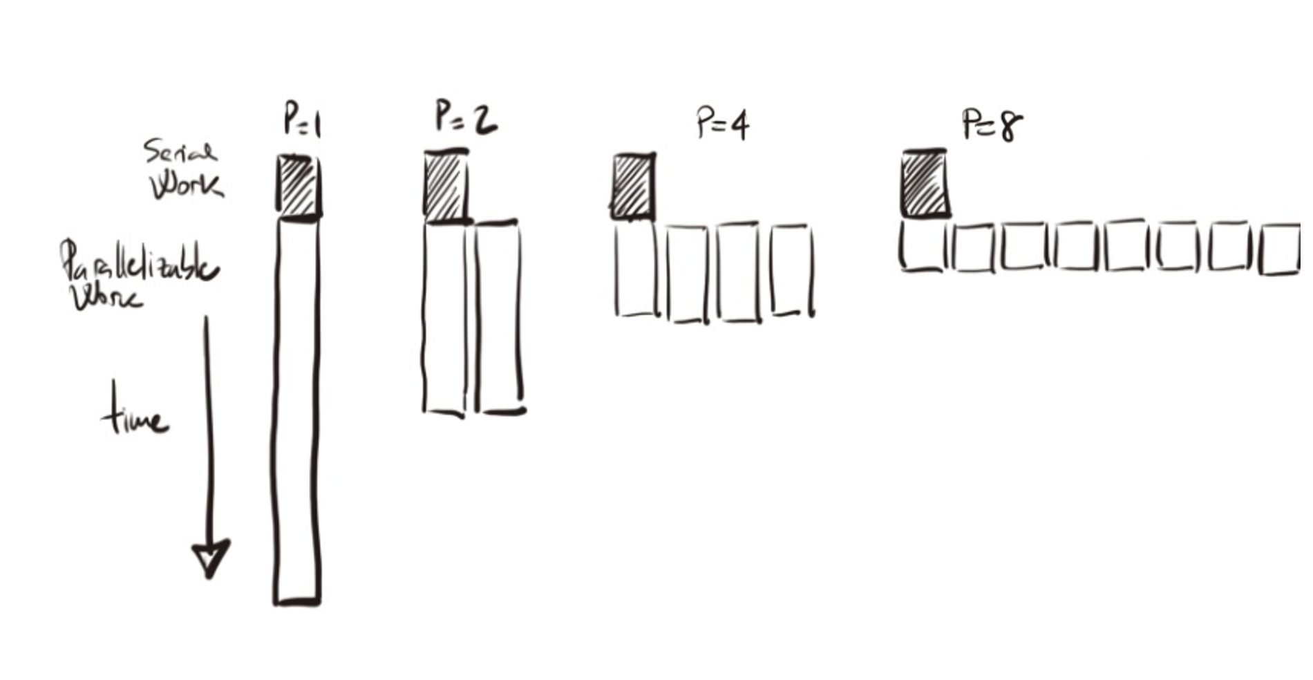
Figure 1.13 – Amdahl’s Law: Speedup is limited by the non-parallelizable serial portion of the work.*

Suppose that we are able to parallelize 90% of a serial program and the speedup of the parallel part is linear regardless of the number of execution units we use. The remaining 10 percent of the execution time is spent in functions that must be executed sequentially on a single execution unit. What is the maximum speedup that we could expect from a parallel version of the program executing on eight processing units?

We apply Amdahl’s Law and obtain:

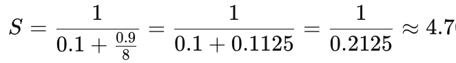
The maximum speedup expected with 8 processors is approximately 4.7.

Amdahl’s Law can also be used to determine the asymptotic speedup achievable as the number of execution units increases. Even with an infinite number of processing units, the maximum speedup is limited by the sequential portion of the workload:

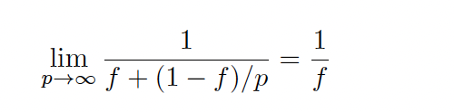
In Figure 1.14 we can visualize a schematic illustration of the speedup against the number of processing units. With this illustration we want to remark the impact of f in the maximum speedup limited. Speedup flattens quickly as p increases, especially if f is non-negligible. This law highlights that improving sequential code remains essential.

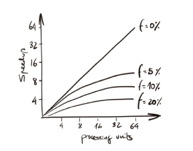
Figure 1.14 – Speedup against the number of processors: *f represents the fraction of the computation that cannot be divided into concurrent tasks.*

Imagine that we have measured the execution times of the sequential version of a matrix-vector multiplication program. The serial part takes 49.13 microseconds, while the parallel portion takes 2.90 microseconds. What is the maximum speedup we could expect from a parallel version of the program running on a high performance parallel supercomputer?

The total execution time is 49.13 + 2.90 = 52.03 microseconds. The serial fraction of the code is 49/52.03 ≈ 0.944. Therefore, the maximum theoretical speedup as the number of processors tends to infinity is 1/0.944 ≈ 1.059.

This result illustrates a case where parallelization offers little performance improvement because most of the execution time is spent in the serial portion of the code.

We can clearly observe much larger speedups in today’s programs than Gene Amdahl originally anticipated in his seminal paper, likely because his assumption about the inherently sequential fraction of the program was overly conservative. This is largely due to the fact that the premises and elements of his equation no longer fully apply in modern parallel computing environments.
Over time, we have learned how to design highly parallel programs, and as we scale up problem sizes, the fraction of parallelizable work often increases — sometimes almost without bound. We will analyze this situation further in the next section, when we introduce Gustafson-Barsis’s Law.

Furthermore, Amdahl’s Law assumes that performance improvement from adding processors is strictly a linear function of the number of processors. However, many additional factors influence actual performance. For example, building larger caches may improve performance for certain problems even more effectively than simply adding processing units, allowing speedups beyond those predicted by Amdahl’s Law.

In addition, Amdahl’s Law presumes that all processing units are identical. In contrast, modern heterogeneous accelerated systems often combine a host with a small number of general-purpose CPU cores and a highly parallel accelerator with many cores of a different architecture.

In summary, the assumptions underlying Amdahl’s Law no longer fully reflect the performance characteristics of modern supercomputing systems, where many of its simplifying conditions are no longer valid. Nevertheless, we include it in this book because this simple and elegant performance model remains one of the most frequently cited works in the field of parallel computing, and it provides an excellent starting point for students to reflect on the performance limits of parallel programs.

Task 1.3 – Applying Amdahl’s Law

Suppose you have a program in which 85% of the code can be parallelized. Use Amdahl’s Law to compute the maximum theoretical speedup when using 4,8,16, 64 and an infinite number of processing units.

What do you observe? Explain why this happens and why it matters in real-world scenarios.

Gustafson-Barsis’s Law

Amdahl’s Law assumes that the problem size is fixed and analyzes how performance improves as the number of processing units increases. However, in practice, this assumption often does not hold: as computing resources become available, applications typically scale up to address larger problem sizes.

More than two decades after the formulation of Amdahl’s Law, John Gustafson (in 1988) identified this limitation and proposed an alternative perspective that better reflects empirical observations in many real-world scenarios.

Gustafson observed that in many cases, the parallel portion of the computation grows substantially as the problem size increases, while the serial portion either remains constant or grows much more slowly. Consequently, the serial fraction becomes progressively smaller relative to the total execution time (as visually illustrated in Figure 1.15).

This insight leads to a different performance model: scaled speedup, in which speedup is measured by solving a larger problem in the same amount of time while utilizing more processors. Under this model, speedup can increase nearly linearly with the number of processors, provided that the serial fraction remains sufficiently small.

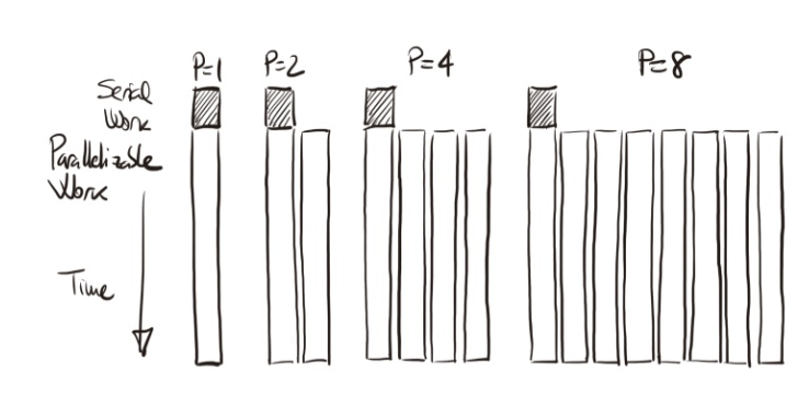
Figure 1.15 – Illustration of scaled speedup based on the same example as in Figure 1.13. As the problem size grows with *p, the parallel portion scales proportionally while the serial part remains constant, reducing the serial fraction and increasing speedup.*

This behavior can be further illustrated by examining how different types of algorithms scale with problem size. In many applications, inherently sequential components such as data input or output tend to grow proportionally to the size of the problem. In contrast, the computational workload often grows much faster. For example, certain sorting algorithms require a number of operations that increases roughly with the square of the problem size, while matrix multiplication requires a number of operations that increases approximately with the cube of the problem size. As a result, increasing the problem size leads to a disproportionate growth in the parallel workload relative to the serial portion, making the serial fraction progressively smaller and allowing parallel efficiency to improve as more processors are utilized.

Gustafson-Barsis’s Law can be formalized as follows: given a parallel program executed on p processing units, let s denote the fraction of total execution time spent in the serial portion of the code. Then, the maximum speedup achievable is given by:

p − s(p − 1)

This formulation reflects a more realistic model for modern parallel computing environments, where increasing the number of processing units is often accompanied by a proportional increase in problem size. The result is a scaled speedup model, where parallel systems are not used merely to solve a fixed problem faster, but rather to handle larger or more complex problems within the same execution time.

As an example, consider a matrix-vector multiplication algorithm executed using 32 processors. The benchmarking indicates that 37% of this time is spent executing the serial portion of the computation on a single processing unit. We want to determine the maximum speedup achievable for this application according to Gustafson-Barsis’s Law. Applying the formula:

32-0.37(32-1) =20.53

Therefore, we should expect a maximum speedup of approximately 20.53 for this application.

In summary, Gustafson’s Law also provides an upper bound for the speedup that can be expected from a parallel version of a given program. It is important to note, however, that this law does not account for communication overhead, which can significantly affect real-world performance.

Task 1.4 – Gustafson-Barsis’s Law and Scaling Intuition

Let’s assume a program is executed on 32 processors. You measure that 30% of the execution time is spent in serial work. Using Gustafson-Barsis’s Law, calculate the maximum speedup. Now, suppose the problem size increases proportionally with the number of processors. What happens to the serial fraction?

Reflect on why this scaling behavior is often more realistic in scientific applications than what Amdahl’s Law predicts.

Explain your reasoning and discuss why this result aligns with the scaling behavior observed in real scientific workloads.

Parallel Overhead and the Limits of Speedup Models

While Amdahl’s and Gustafson-Barsis’s laws provide useful first-order models for understanding the theoretical limits of speedup in parallel computing, they both rely on highly idealized assumptions. In practice, many real-world factors limit the achievable performance of parallel systems. These limitations are often grouped under the general concept of parallel overhead, which refers to all additional work or delays introduced as a consequence of managing parallel execution.

Parallel overhead can stem from a variety of sources, each contributing to deviations from ideal speedup behavior. The most common forms of parallel overhead encountered in supercomputing environments:

• Communication Overhead: In parallel systems, tasks frequently need to exchange data among processing units. This communication occurs both within nodes (e.g., shared memory or cache transfers) and across nodes (e.g., message passing over interconnects). The time spent on these data transfers can grow significantly as the number of processors increases or as the problem size becomes large.

• Synchronization Overhead: Many parallel algorithms require synchronization points where multiple threads or processes must wait for each other to reach the same stage of execution before proceeding. These barriers introduce idle time whenever some processing units complete their tasks earlier than others.

• Load Imbalance: Load imbalance occurs when work is unevenly distributed among processing units, causing some processors to idle while others continue executing longer tasks. Even if the total work is parallelizable, poor workload distribution leads to inefficient resource utilization.

• Startup Overhead: Startup overhead refers to the time required to initialize parallel resources, allocate memory, launch threads or processes, and establish communication contexts. While startup costs are often negligible for long-running computations, they can be significant for short or fine-grained parallel tasks.

• Memory and Cache Effects: Memory hierarchy behavior can introduce additional overheads that are not directly captured by classical speedup models.

• Operating System and Runtime Overheads: System-level factors such as operating system scheduling, thread management, and runtime library overheads can introduce additional delays.

Effective parallel programming requires not only maximizing parallel work but also minimizing the many sources of overhead that prevent ideal scalability. Many of these issues related to parallel overhead and scalability will be examined in greater detail throughout the practical case studies presented in the later chapters of this book.

Key Takeaways from Chapter 1

• In this book, we will use the terms supercomputing and high performance computing (HPC) interchangeably, referring to the fundamental discipline of designing and using powerful computing systems to solve complex problems efficiently.

• Supercomputers are essential tools for tackling problems that are both computationally intensive and data-heavy, such as climate modeling, biomedical simulations, or training large-scale AI models. These systems are not simply faster versions of regular computers—they are architected specifically to exploit parallelism.

• Parallelism is the cornerstone of HPC. Achieving high speedup requires dividing a problem into independent tasks that can be executed simultaneously.

• Peak performance is often far from the sustained performance achieved in real applications. This gap arises due to limitations in memory bandwidth, communication latency, and software efficiency. Benchmark suites such as HPL are used to generate the Top500 list, which ranks worldwide HPC systems based on FLOPS.

• Energy consumption has become a first-class concern in HPC. As supercomputers grow in scale and complexity, minimizing power usage while maximizing useful computation becomes essential—for both environmental and economic reasons. The Green500 list ranks supercomputers according to their energy efficiency.

• Performance metrics such as speedup, efficiency, and scalability help quantify how well a program benefits from parallelization. Speedup compares execution times, efficiency relates the gain to the number of processors used, and scalability describes how performance evolves as computational resources increase. Amdahl’s and Gustafson’s laws serve as useful tools for building intuition and performing quick preliminary estimates to evaluate scalability under idealized conditions.

• Achieving good parallel performance in practice is not trivial. Overheads such as inter-process communication, task synchronization, and workload imbalance can significantly reduce the benefits of adding more processors. Understanding these performance degradation factors is essential for writing efficient parallel code.

1. In this part of the book, processing units refers broadly to CPUs, cores, and GPU accelerators, in order to generalize before introducing more precise terminology later on. ↩

2. In this book, the terms serial and sequential are closely related but not identical. Sequential refers to any execution where instructions are carried out one after another, regardless of whether parallel execution would be possible. In contrast, serial typically refers to the inherently non-parallelizable part of a program—that is, the portion that must be executed in sequence and cannot benefit from parallel execution. When describing program execution on a single processing unit, both terms may be used interchangeably in this book for simplicity, unless a precise distinction is required by context. ↩

3. In the context of HPC, throughput refers to the number of useful operations completed per unit of time, reflecting how effectively a supercomputer utilizes its computational resources. ↩

4. https://top500.org/ ↩